05 | Introduction to Data Science

Python data workflows with Polars and Plotly

Author

Affiliation

Mr. Ozan Ozbeker

Industrial and Management Systems Engineering

1 Overview

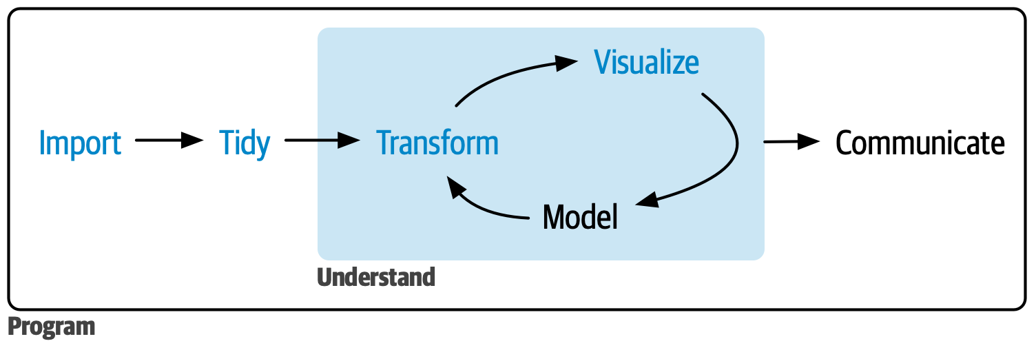
In this beginning chapter, we will cover the fundamentals of data analysis in the form of importing, tidying, transforming, and visualizing data, as shown below:

In this learning module, you’ll learn how to import, tidy, transform, and visualize data.

By the end of this module, you will be able to:

• Import data from various file formats into Python using Polars
• Clean and reshape datasets to facilitate analysis
• Transform data through filtering, sorting, and creating new variables
• Group and aggregate data to identify patterns and trends
• Visualize distributions and relationships using Plotly Express
• Apply tidy data principles to structure datasets effectively

1.1 Initialization

At this point, you will need to install a few more Python packages:

terminal

uv add polars[all] plotly[express] statsmodels palmerpenguins nycflights13

Once installed, import the following:

import plotly.express as px
import polars as pl
import polars.selectors as cs
import palmerpenguins
import nycflights13

2 Data visualization

Python has several systems for making graphs, but we will be focusing on Plotly, specifically Plotly Express. Plotly Express contains functions that can create entire plots at once, and makes it easy to create most common figures.

This section will teach you how to visualize your data using Plotly Express, walking through visualizing distributions of single variables, as well as relationships between two or more variables.

2.1 The penguins data frame

The dataset we will be working with is a commonly used one, affectionately referred to as the Palmer Penguins, which includes body measurements for penguins on three islands in the Palmer Archipelago. A data frame is a rectangular collection of variables (in the columns) and observations (in the rows). penguins contains 344 observations collected and made available by Dr. Kristen Gorman and the Palmer Station, Antarctica.

Let’s define some term:

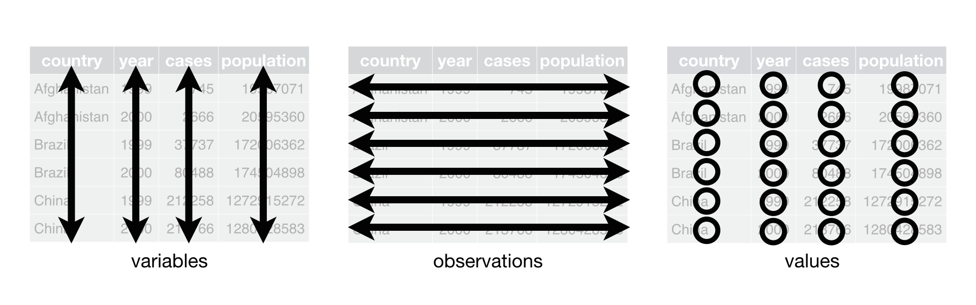
• A variable is a quantity, quality, or property that you can measure.
• A value is the state of a variable when you measure it. The value of a variable may change from measurement to measurement.
• An observation is a set of measurements made under similar conditions (you usually make all of the measurements in an observation at the same time and on the same object). An observation will contain several values, each associated with a different variable. We’ll sometimes refer to an observation as a data point.
• Tabular data is a set of values, each associated with a variable and an observation. Tabular data is tidy if each value is placed in its own “cell”, each variable in its own column, and each observation in its own row.

In this context, a variable refers to an attribute of all the penguins, and an observation refers to all the attributes of a single penguin.

We will use palmerpenguins package to get the penguins data, and convert it to a polars data frame:

penguins = pl.from_pandas(palmerpenguins.load_penguins())

The reason we convert to a Polars data frame is because we want to use the tools and methods that come with Polars:

type(penguins)

polars.dataframe.frame.DataFrame

Depending on what tool/IDE you’re using Python with, just having the variable name (penguins) as the last line will print a formatted view of the data. If not, you can also use print() to use Polars’ native formatting:

penguins

shape: (344, 8)

species	island	bill_length_mm	bill_depth_mm	flipper_length_mm	body_mass_g	sex	year
str	str	f64	f64	f64	f64	str	i64
"Adelie"	"Torgersen"	39.1	18.7	181.0	3750.0	"male"	2007
"Adelie"	"Torgersen"	39.5	17.4	186.0	3800.0	"female"	2007
"Adelie"	"Torgersen"	40.3	18.0	195.0	3250.0	"female"	2007
"Adelie"	"Torgersen"	null	null	null	null	null	2007
…	…	…	…	…	…	…	…
"Chinstrap"	"Dream"	43.5	18.1	202.0	3400.0	"female"	2009
"Chinstrap"	"Dream"	49.6	18.2	193.0	3775.0	"male"	2009
"Chinstrap"	"Dream"	50.8	19.0	210.0	4100.0	"male"	2009
"Chinstrap"	"Dream"	50.2	18.7	198.0	3775.0	"female"	2009

print(penguins)

shape: (344, 8)
┌───────────┬───────────┬──────────────┬──────────────┬──────────────┬─────────────┬────────┬──────┐
│ species   ┆ island    ┆ bill_length_ ┆ bill_depth_m ┆ flipper_leng ┆ body_mass_g ┆ sex    ┆ year │
│ ---       ┆ ---       ┆ mm           ┆ m            ┆ th_mm        ┆ ---         ┆ ---    ┆ ---  │
│ str       ┆ str       ┆ ---          ┆ ---          ┆ ---          ┆ f64         ┆ str    ┆ i64  │
│           ┆           ┆ f64          ┆ f64          ┆ f64          ┆             ┆        ┆      │
╞═══════════╪═══════════╪══════════════╪══════════════╪══════════════╪═════════════╪════════╪══════╡
│ Adelie    ┆ Torgersen ┆ 39.1         ┆ 18.7         ┆ 181.0        ┆ 3750.0      ┆ male   ┆ 2007 │
│ Adelie    ┆ Torgersen ┆ 39.5         ┆ 17.4         ┆ 186.0        ┆ 3800.0      ┆ female ┆ 2007 │
│ Adelie    ┆ Torgersen ┆ 40.3         ┆ 18.0         ┆ 195.0        ┆ 3250.0      ┆ female ┆ 2007 │
│ Adelie    ┆ Torgersen ┆ null         ┆ null         ┆ null         ┆ null        ┆ null   ┆ 2007 │
│ …         ┆ …         ┆ …            ┆ …            ┆ …            ┆ …           ┆ …      ┆ …    │
│ Chinstrap ┆ Dream     ┆ 43.5         ┆ 18.1         ┆ 202.0        ┆ 3400.0      ┆ female ┆ 2009 │
│ Chinstrap ┆ Dream     ┆ 49.6         ┆ 18.2         ┆ 193.0        ┆ 3775.0      ┆ male   ┆ 2009 │
│ Chinstrap ┆ Dream     ┆ 50.8         ┆ 19.0         ┆ 210.0        ┆ 4100.0      ┆ male   ┆ 2009 │
│ Chinstrap ┆ Dream     ┆ 50.2         ┆ 18.7         ┆ 198.0        ┆ 3775.0      ┆ female ┆ 2009 │
└───────────┴───────────┴──────────────┴──────────────┴──────────────┴─────────────┴────────┴──────┘

This data frame contains 8 columns. For an alternative view, use DataFrame.glimpse(), which is helpful for wide tables that have many columns:

penguins.glimpse()

Rows: 344
Columns: 8
$ species           <str> 'Adelie', 'Adelie', 'Adelie', 'Adelie', 'Adelie', 'Adelie', 'Adelie', 'Adelie', 'Adelie', 'Adelie'
$ island            <str> 'Torgersen', 'Torgersen', 'Torgersen', 'Torgersen', 'Torgersen', 'Torgersen', 'Torgersen', 'Torgersen', 'Torgersen', 'Torgersen'
$ bill_length_mm    <f64> 39.1, 39.5, 40.3, None, 36.7, 39.3, 38.9, 39.2, 34.1, 42.0
$ bill_depth_mm     <f64> 18.7, 17.4, 18.0, None, 19.3, 20.6, 17.8, 19.6, 18.1, 20.2
$ flipper_length_mm <f64> 181.0, 186.0, 195.0, None, 193.0, 190.0, 181.0, 195.0, 193.0, 190.0
$ body_mass_g       <f64> 3750.0, 3800.0, 3250.0, None, 3450.0, 3650.0, 3625.0, 4675.0, 3475.0, 4250.0
$ sex               <str> 'male', 'female', 'female', None, 'female', 'male', 'female', 'male', None, None
$ year              <i64> 2007, 2007, 2007, 2007, 2007, 2007, 2007, 2007, 2007, 2007

Among these variables are:

1. species: a penguin’s species (Adelie, Chinstrap, or Gentoo).
2. flipper_length_mm: length of a penguin’s flipper, in millimeters.
3. body_mass_g: body mass of a penguin, in grams.

2.2 First visualization

Our goal is to recreate the following visual that displays the relationship between flipper lengths and body masses of these penguins, taking into consideration the species of the penguin.

2.3 Using Plotly Express

With Plotly Express, you begin a plot by calling a plotting function from the module, commonly referred to as px. You can then add arguments to your plot function for more customization.

At it’s most basic form, the plotting function creates a blank canvas with a grid since we’ve given it no data.

px.scatter()

Next, we need to actually provide data, along with the appropriate number of variables depending on the type of plot we are trying to create.

px.scatter(data_frame=penguins, x="flipper_length_mm", y="body_mass_g")

px.scatter() creates a scatter plot, and we will learn many more plot types through out the course. You can learn more about the different plots Plotly Express offers at their gallery.

This doesn’t match our “final goal” yet, but using this plot we can start answering the question that motivated our exploration: “What does the relationship between flipper length and body mass look like?” The relationship appears to be positive (as flipper length increases, so does body mass), fairly linear (the points are clustered around a line instead of a curve), and moderately strong (there isn’t too much scatter around such a line). Penguins with longer flippers are generally larger in terms of their body mass.

Before we go further, I want to point out that this dataset has some missing values for flipper_length_mm and body_mass_g, but Plotly does not warn you about this when creating the plot. If one and/or other variable is missing data, we cannot plot that.

2.4 Adding aesthetics and layers

Scatter plots are useful for displaying the relationship between two numerical variables, but it’s always a good idea to be skeptical of any apparent relationship between two variables and ask if there may be other variables that explain or change the nature of this apparent relationship. For example, does the relationship between flipper length and body mass differ by species? Let’s incorporate species into our plot and see if this reveals any additional insights into the apparent relationship between these variables. We will do this by representing species with different colored points.

To achieve this, we will use some of the other arguments that px.scatter() provides for us, like color:

px.scatter(
    data_frame=penguins, 
    x="flipper_length_mm", 
    y="body_mass_g", 
    color="species"
)

When a categorical variable is mapped to an aesthetic, Plotly will automatically assign a unique value of the aesthetic (here, a unique color) to each unique level of the variable (each of the three species), a process known as scaling. Plotly will also add a legend that explains which value correspond to which levels.

Now let’s add another layer, a trendline displaying the relationship between body mass and flipper length. px.scatter() has an argument for this, trendline, and a couple other arguments that modify its behavior. Specifically, we want to draw a line of best fit using Ordinary Least Squares (ols). You can see the other options, and more info about this plotting function with ?px.scatter() or in the online documentation.

px.scatter(
    data_frame=penguins, 
    x="flipper_length_mm", 
    y="body_mass_g", 
    color="species",
    trendline="ols"
)

We’ve added lines, but this plot doesn’t look like our final goal, which only has one line for the entire dataset, opposed to separate lines for each of the penguin species. px.scatter() has an argument, trendline_scope, which controls how the trendline is drawn when there are groups, in this case created when we used color="species". The default for trendline_scope is "trace", which draws a line per color, symbol, facet, etc., and "overall", which computes one trendline for the entire dataset,a nd replicates across all facets.

px.scatter(
    data_frame=penguins, 
    x="flipper_length_mm", 
    y="body_mass_g", 
    color="species",
    trendline="ols",
    trendline_scope="overall"
)

Now we have something that is very close to our final plot, thought it’s not there yet. We still need to use different shapes for each species and improve the labels.

It’s generally not a good idea to represent information only using colors on a plot as people perceive colors differently do to color blindness or other color vision difference. px.scatter() allows us to control the shapes of the dots using the symbol argument.

px.scatter(
    penguins,
    x="flipper_length_mm",
    y="body_mass_g",
    color="species",
    symbol="species",
    trendline="ols",
    trendline_scope="overall",
)

Note that the legend is automatically updated to reflect the different shapes of the points as well.

Finally, we can use title, subtitle, and labels arguments to update our labels. title and subtitle just take a string, adding labels are bit more advanced. labels takes a dictionary with key:value combos for each of the labels on the plot that you would like to change. In our plot, we want to update the labels for the x-axis, y-axis, and the legend, but we refer to them by their current label, not their position:

px.scatter(
    penguins,
    x="flipper_length_mm",
    y="body_mass_g",
    color="species",
    symbol="species",
    trendline="ols",
    trendline_scope="overall",
    title="Body mass and flipper length",
    subtitle="Dimensions for Adelie, Chinstrap, and Gentoo Penguins",
    labels={
        "species":"Species",
        "body_mass_g":"Body mass (g)",
        "flipper_length_mm":"Flipper length (mm)"
    }
)

Now we have our final plot. If you haven’t noticed already, Plotly creates interactive plots, you can hover over certain data points to see their values, use the legend as a filter, and so on. In the top right of every plot, you will see a menu with some options.

2.5 Visualizing distributions

How you visualize the distribution of a variable depends on the type of the variable: categorical or numerical.

2.5.1 A categorical variable

A value is categorical if it can only take one of a small set of values. To examine the distribution of a categorical variable, you can use a bar chart. The height of the bars displays how many observations occurred with each x value.

px.bar(penguins, x="species")

px.bar() will result in one rectangle drawn per row of input, which can result in the striped look above. To combine these rectangles into on color per position, we can pre-calculate the count as and use it as the y value:

# we'll learn more about this Polars code later
penguins_count = penguins.group_by("species").len("count")
print(penguins_count)

px.bar(penguins_count, x="species", y="count")

shape: (3, 2)
┌───────────┬───────┐
│ species   ┆ count │
│ ---       ┆ ---   │
│ str       ┆ u32   │
╞═══════════╪═══════╡
│ Adelie    ┆ 152   │
│ Gentoo    ┆ 124   │
│ Chinstrap ┆ 68    │
└───────────┴───────┘

The order of categorical values in axes, legends, and facets depends on the order in which these values are first encountered in data_frame. It’s often preferable to re-order the bars based on their frequency, which we can do with the category_orders argument. category_orders takes a dictionary where the keys correspond to column names, and the values should be lists of strings corresponding to the specific display order desired

px.bar(
    penguins_count,
    x="species", 
    y="count",
    category_orders={"species": ["Adelie", "Gentoo", "Chinstrap"]}
)

While it’s easy enough to manually sort three columns, this could become very tedious for more columns. Here is one programmatic way you could sort the columns:

penguins_sorted = (
    penguins_count
    .sort(by="count", descending=True)
    .get_column("species")
)

print(penguins_sorted)

px.bar(
    penguins_count,
    x="species", 
    y="count",
    category_orders={"species": penguins_sorted}
)

shape: (3,)
Series: 'species' [str]
[
    "Adelie"
    "Gentoo"
    "Chinstrap"
]

We will dive into the data manipulation code later, this is just to show what’s possible.

2.5.2 A numerical variable

A variable is numerical (or quantitative) if it can take on a wide range of numerical values, and it is sensible to add, subtract, or take averages with those values. Numerical variables can be continuous or discrete.

One common visualization for distributions of continuous variables is a histogram.

px.histogram(penguins, x="body_mass_g")

A histogram divides the x-axis into equally spaced bins and then uses the heigh of the bar to display the number observations that fall in each bin. In the graph above, the tallest bar shows that 39 observations have a body_mass_g value between 3,500 and 3,700 grams, which are the left and right edges of the bar.

When working with histograms, it’s a good idea to use different number of bins to reveal different patterns in the data. In the plots below, X bars is too many, resulting in narrow bars. Similarly, 3 bins is too few, resulting in all the data being binned into huge categories that make it difficult to determine the shape of the distribution. A bin number of 20 provides a sensible balance.

px.histogram(penguins, x="body_mass_g", nbins=200)
px.histogram(penguins, x="body_mass_g", nbins=3)
px.histogram(penguins, x="body_mass_g", nbins=20)

An alternative visualization for distributions of numerical variables is a density plot. A density plot is a smoothed-out version of a histogram and a practical alternative, particularly for continuous data that comes from an underlying smooth distribution. At the time of writing, Plotly Express doesn’t have a quick way to create a density plot, but it does offer very customizable violin plots, which we can make to look like a density plot if we would like.

px.violin(penguins, x="body_mass_g")

The density plot is similar to the violin plot, with only one side, and the peaks are more exaggerated:

px.violin(
    penguins, 
    x="body_mass_g", # plots the variable across the x-axis
    range_y=[
        0,   # limits the bottom of y-axis, removing reflection
        0.25 # limits the top of y-axis, stretching the peaks
    ]
)

While this workaround works, sticking to the original violin plot I think looks better, and we can add some extra arguments to see more details:

px.violin(penguins, x="body_mass_g", points="all")

Play around with different arguments and see what you like best!

As an analogy to understand these plots vs a histogram, imagine a histogram made out of wooden blocks. Then, imagine that you drop a cooked spaghetti string over it. The shape the spaghetti will take draped over blocks can be thought of as the shape of the density curve. It shows fewer details than a histogram but can make it easier to quickly glean the shape of the distribution, particularly with respect to modes and skewness.

2.6 Visualizing relationships

To visualize a relationship we need to have at least two variables mapped to aesthetics of a plot. In the following sections you will learn about commonly used plots for visualizing relationships between two or more variables and the plots used for creating them.

2.6.1 A numerical and a categorical variable

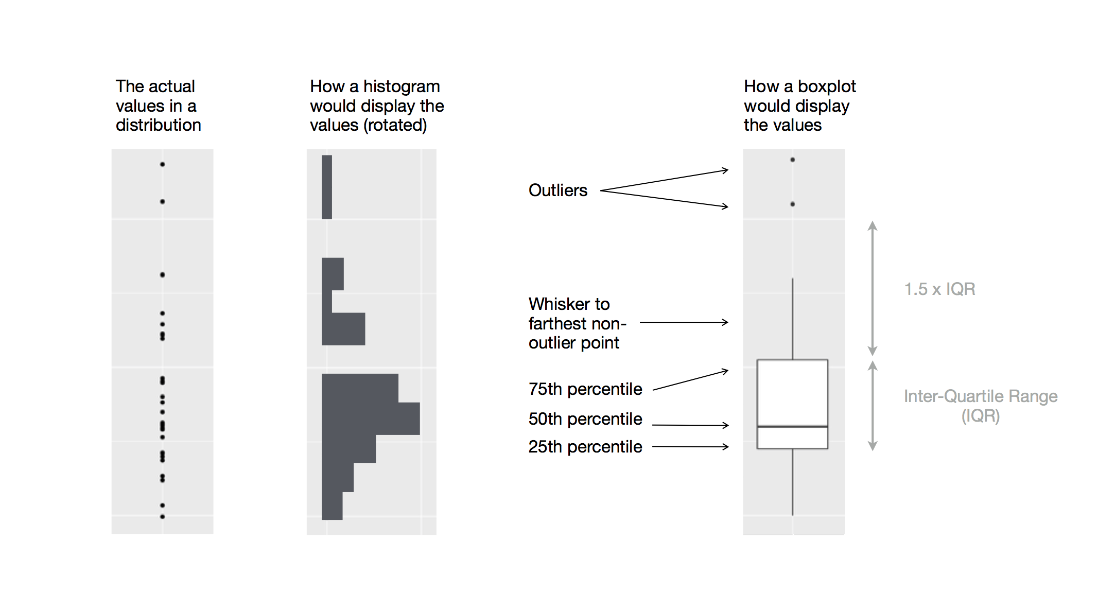
To visualize the relationship between a numerical and a categorical variable we can use side-by-side box plots. A boxplot is a type of visual shorthand for measures of position (percentiles) that describe a distribution. It is also useful for identifying potential outliers. Each boxplot consists of:

• A box that indicates the range of the middle half of the data, a distance known as the inter-quartile range (IQR), stretching from the 25th percentile of the distribution to the 75th percentile. In the middle of the box is a line that displays the median, i.e. 50th percentile, of the distribution. These three lines give you a sense of the spread of the distribution and whether or not the distribution is symmetric about the median or skewed to one side.

• Visual points that display observations that fall more than 1.5 times the IQR from either edge of the box. These outlying points are unusual so are plotted individually.

• A line (or whisker) that extends from each end of the box and goes to the farthest non-outlier point in the distribution.

“Diagram depicting how a boxplot is created.”

Let’s take a look at the distribution of body mass by species using px.box()

px.box(penguins, x="species", y="body_mass_g")

Alternatively, we can make violin plots with multiple groups:

px.violin(penguins, x="body_mass_g", color="species", box=True)

As we’ve seen before, there are many ways to see and code what we are looking for.

2.6.2 Two categorical variables

We can use stacked bar plots to visualize the relationship between two categorical variables. For example, the following two stacked bar plots both display the relationship between island and species, or specifically, visualizing the distribution of species within each island.

The first plot shows the frequencies of each species of penguins on each island. The plot of frequencies shows that there are equal numbers of Adelies on each island. But we don’t have a good sense of the percentage balance within each island.

px.bar(penguins, x="island", color="species")

or

data = penguins.group_by(["island", "species"]).len("count")
data_order = data.group_by("island").agg(pl.col("count").sum()).sort(by="count", descending=True).get_column("island")


px.bar(
    data, x="island", y="count", color="species",
    category_orders = {"island": data_order, "species": data_order}
)

2.6.3 Two numerical variables

So far we’ve seen scatter plots for visualizing the relationship between two numerical variables. A scatter plot is probably the most commonly used plot for visualizing the relationship between to numerical variables.

px.scatter(penguins, x="flipper_length_mm", y="body_mass_g")

2.6.4 Three or more variables

As we saw before, we can incorporate more variables into a plot by mapping them to additional aesthetics. For example, in the following plot, the colors of points represent species and the shapes represent islands.

px.scatter(
    penguins, 
    x="flipper_length_mm", y="body_mass_g",
    color="species", symbol="island"
)

However adding too many aesthetic mappings to a plot makes it cluttered and difficult to make sense of. Another way, which is particularly useful for categorical variables, is to split your plot into facets, subplots that each display one subset of the data.

Most Plotly Express functions provide arguments to facet, just make sure to check the documentation.

px.scatter(
    penguins, 
    x="flipper_length_mm", y="body_mass_g",
    color="species", symbol="island",
    facet_col="island"
)

2.7 Summary

In this section, you’ve learned the basics of data visualization with Plotly Express. We started with the basic idea that underpins Plotly Express: a visualization is a mapping from variables in your data to aesthetic properties like position, color, size and shape. You then learned about increasing the complexity with more arguments in the Plotly functions. You also learned about commonly used plots for visualizing the distribution of a single variable as well as for visualizing relationships between two or more variables, by leveraging additional aesthetic mappings and/or splitting your plot into small multiples using faceting.

3 Data transformation

Visualization is an important tool for generating insight, but it’s rare that you get the data in exactly the right form you need to make the graph you want. Often you’ll need to create some new variables or summaries to answer your questions with your data, or maybe you just want to rename the variables or reorder the observations to make the data a little easier to work with. We’ve already seen examples of this above when creating the bar charts. In this section, we’ll see how to do that with the Polars package.

The goal of this section is to give you an overview of all the key tools for transforming a data frame. We’ll start with functions that operate on rows and then columns of a data frame, then circle back to talk more about method chaining, an important tool that you use to combine functions. We will then introduce the ability to work with groups. We will end the section with a case study that showcases these functions in action.

3.1 The flights data frame

To explore basic Polars methods and expressions, we will use the flights data frame from the nycflights13 package. This dataset contains all 336,776 flights that departed from New York City in 2013.

flights = (
    pl.from_pandas(nycflights13.flights)
    .with_columns(pl.col("time_hour").str.to_datetime("%FT%TZ"))
) # We will learn what's going on here in later this section

flights

shape: (336_776, 19)

year	month	day	dep_time	sched_dep_time	dep_delay	arr_time	sched_arr_time	arr_delay	carrier	flight	tailnum	origin	dest	air_time	distance	hour	minute	time_hour
i64	i64	i64	f64	i64	f64	f64	i64	f64	str	i64	str	str	str	f64	i64	i64	i64	datetime[μs]
2013	1	1	517.0	515	2.0	830.0	819	11.0	"UA"	1545	"N14228"	"EWR"	"IAH"	227.0	1400	5	15	2013-01-01 10:00:00
2013	1	1	533.0	529	4.0	850.0	830	20.0	"UA"	1714	"N24211"	"LGA"	"IAH"	227.0	1416	5	29	2013-01-01 10:00:00
2013	1	1	542.0	540	2.0	923.0	850	33.0	"AA"	1141	"N619AA"	"JFK"	"MIA"	160.0	1089	5	40	2013-01-01 10:00:00
2013	1	1	544.0	545	-1.0	1004.0	1022	-18.0	"B6"	725	"N804JB"	"JFK"	"BQN"	183.0	1576	5	45	2013-01-01 10:00:00
…	…	…	…	…	…	…	…	…	…	…	…	…	…	…	…	…	…	…
2013	9	30	null	2200	null	null	2312	null	"9E"	3525	null	"LGA"	"SYR"	null	198	22	0	2013-10-01 02:00:00
2013	9	30	null	1210	null	null	1330	null	"MQ"	3461	"N535MQ"	"LGA"	"BNA"	null	764	12	10	2013-09-30 16:00:00
2013	9	30	null	1159	null	null	1344	null	"MQ"	3572	"N511MQ"	"LGA"	"CLE"	null	419	11	59	2013-09-30 15:00:00
2013	9	30	null	840	null	null	1020	null	"MQ"	3531	"N839MQ"	"LGA"	"RDU"	null	431	8	40	2013-09-30 12:00:00

flights is a Polars DataFrame. Different packages have their own version of a data frame with their own methods, functions, etc., but in this course, we will be using Polars. Polars provides its own way of working with data frames, as well as importing, exporting, printing, and much more, including the previously shown DataFrame.glimpse() method:

flights.glimpse()

Rows: 336776
Columns: 19
$ year                    <i64> 2013, 2013, 2013, 2013, 2013, 2013, 2013, 2013, 2013, 2013
$ month                   <i64> 1, 1, 1, 1, 1, 1, 1, 1, 1, 1
$ day                     <i64> 1, 1, 1, 1, 1, 1, 1, 1, 1, 1
$ dep_time                <f64> 517.0, 533.0, 542.0, 544.0, 554.0, 554.0, 555.0, 557.0, 557.0, 558.0
$ sched_dep_time          <i64> 515, 529, 540, 545, 600, 558, 600, 600, 600, 600
$ dep_delay               <f64> 2.0, 4.0, 2.0, -1.0, -6.0, -4.0, -5.0, -3.0, -3.0, -2.0
$ arr_time                <f64> 830.0, 850.0, 923.0, 1004.0, 812.0, 740.0, 913.0, 709.0, 838.0, 753.0
$ sched_arr_time          <i64> 819, 830, 850, 1022, 837, 728, 854, 723, 846, 745
$ arr_delay               <f64> 11.0, 20.0, 33.0, -18.0, -25.0, 12.0, 19.0, -14.0, -8.0, 8.0
$ carrier                 <str> 'UA', 'UA', 'AA', 'B6', 'DL', 'UA', 'B6', 'EV', 'B6', 'AA'
$ flight                  <i64> 1545, 1714, 1141, 725, 461, 1696, 507, 5708, 79, 301
$ tailnum                 <str> 'N14228', 'N24211', 'N619AA', 'N804JB', 'N668DN', 'N39463', 'N516JB', 'N829AS', 'N593JB', 'N3ALAA'
$ origin                  <str> 'EWR', 'LGA', 'JFK', 'JFK', 'LGA', 'EWR', 'EWR', 'LGA', 'JFK', 'LGA'
$ dest                    <str> 'IAH', 'IAH', 'MIA', 'BQN', 'ATL', 'ORD', 'FLL', 'IAD', 'MCO', 'ORD'
$ air_time                <f64> 227.0, 227.0, 160.0, 183.0, 116.0, 150.0, 158.0, 53.0, 140.0, 138.0
$ distance                <i64> 1400, 1416, 1089, 1576, 762, 719, 1065, 229, 944, 733
$ hour                    <i64> 5, 5, 5, 5, 6, 5, 6, 6, 6, 6
$ minute                  <i64> 15, 29, 40, 45, 0, 58, 0, 0, 0, 0
$ time_hour      <datetime[μs]> 2013-01-01 10:00:00, 2013-01-01 10:00:00, 2013-01-01 10:00:00, 2013-01-01 10:00:00, 2013-01-01 11:00:00, 2013-01-01 10:00:00, 2013-01-01 11:00:00, 2013-01-01 11:00:00, 2013-01-01 11:00:00, 2013-01-01 11:00:00

In both views, the variable names are followed by abbreviations that tell you the type of each variable: i64 is short for integer, f64 is short for float, str is short for string, and datetime[μs] for date-time (in this case, down to the micro-seconds).

We’re going to learn the primary methods (or contexts as Polars calls them) which will allow yo uto solve the vast majority of your data manipulation challenges. Before we discuss their individual differences, it’s worth stating what they have in common:

1. The methods are always attached (or chained) to a data frame.
2. The arguments typically describe which columns to operate on.
3. The output is a new data frame (for the most part, ex: group_by).

Because each method does one thing well, solving complex problems will usually require combining multiple methods, and we will do so with something called “method chaining”. You’ve already seen this before, this is when we attach multiple methods together without creating a placeholder variable between steps. You can think of each . operator of saying “then”. This should help you get a sense of the following code without understanding the details:

flights.filter(
    pl.col("dest") == "IAH"
).group_by(
    ["year", "month", "day"]
).agg( # "aggregate", or summarize
    arr_delay=pl.col("arr_delay").mean()
)

shape: (365, 4)

year	month	day	arr_delay
i64	i64	i64	f64
2013	9	8	-21.5
2013	5	27	-25.095238
2013	11	29	-25.384615
2013	7	17	14.7
…	…	…	…
2013	9	19	2.0
2013	5	1	-2.473684
2013	4	9	-1.526316
2013	3	3	-36.65

We can also write the previous code in a cleaner format. When surrounded by parenthesis, the . operator does not have to “touch” the closing method before it:

(
    flights
    .filter(pl.col("dest") == "IAH")
    .group_by(["year", "month", "day"])
    .agg(arr_delay=pl.col("arr_delay").mean())
)

If we didn’t use method chaining, we would have to create a bunch of intermediate objects:

flights1 = flights.filter(pl.col("dest") == "IAH")
flights2 = flights1.group_by(["year", "month", "day"])
flights3 = flights2.agg(arr_delay=pl.col("arr_delay").mean())

While all of these have their time and place, method chaining generally produces data analysis code that is easier to write and read.

We can organize these contexts (methods) based on what they operate on: rows, columns, groups, or tables.

3.2 Rows

The most important contexts that operate on rows of a dataset are DataFrame.filter(), which changes which rows are present without changing their order, and DataFrame.sort(), which changes the order of the rows without changing which are present. Both methods only affect the rows, and the columns are left unchanged. We’ll also see DataFrame.unique() which returns rows with unique values. Unlike DataFrame.sort() and DataFrame.filter(), it can also optionally modify the columns.

3.2.1 DataFrame.filter()

DataFrame.filter() allows you to keep rows based on the values of the columns. The arguments (also known as predicates) are the conditions that must be true to keep the row. For example, we could find all flights that departed more than 120 minutes late:

flights.filter(pl.col("dep_delay") > 120)

shape: (9_723, 19)

year	month	day	dep_time	sched_dep_time	dep_delay	arr_time	sched_arr_time	arr_delay	carrier	flight	tailnum	origin	dest	air_time	distance	hour	minute	time_hour
i64	i64	i64	f64	i64	f64	f64	i64	f64	str	i64	str	str	str	f64	i64	i64	i64	datetime[μs]
2013	1	1	848.0	1835	853.0	1001.0	1950	851.0	"MQ"	3944	"N942MQ"	"JFK"	"BWI"	41.0	184	18	35	2013-01-01 23:00:00
2013	1	1	957.0	733	144.0	1056.0	853	123.0	"UA"	856	"N534UA"	"EWR"	"BOS"	37.0	200	7	33	2013-01-01 12:00:00
2013	1	1	1114.0	900	134.0	1447.0	1222	145.0	"UA"	1086	"N76502"	"LGA"	"IAH"	248.0	1416	9	0	2013-01-01 14:00:00
2013	1	1	1540.0	1338	122.0	2020.0	1825	115.0	"B6"	705	"N570JB"	"JFK"	"SJU"	193.0	1598	13	38	2013-01-01 18:00:00
…	…	…	…	…	…	…	…	…	…	…	…	…	…	…	…	…	…	…
2013	9	30	1951.0	1649	182.0	2157.0	1903	174.0	"EV"	4294	"N13988"	"EWR"	"SAV"	95.0	708	16	49	2013-09-30 20:00:00
2013	9	30	2053.0	1815	158.0	2310.0	2054	136.0	"EV"	5292	"N600QX"	"EWR"	"ATL"	91.0	746	18	15	2013-09-30 22:00:00
2013	9	30	2159.0	1845	194.0	2344.0	2030	194.0	"9E"	3320	"N906XJ"	"JFK"	"BUF"	50.0	301	18	45	2013-09-30 22:00:00
2013	9	30	2235.0	2001	154.0	59.0	2249	130.0	"B6"	1083	"N804JB"	"JFK"	"MCO"	123.0	944	20	1	2013-10-01 00:00:00

We can use all of the same boolean expressions we’ve learned previous, as well as chain them with & (instead of and), | (instead of or), and ~ (instead of not). Note that Polars is picky about ambiguity, so each condition we check for also has it’s own parenthesis, similar to what we might use in a calculator to make sure the order of operations is being followed exactly as we want:

# Flights that departed on January 1
flights.filter(
    (pl.col("month") == 1) & (pl.col("day") == 1)
)

shape: (842, 19)

year	month	day	dep_time	sched_dep_time	dep_delay	arr_time	sched_arr_time	arr_delay	carrier	flight	tailnum	origin	dest	air_time	distance	hour	minute	time_hour
i64	i64	i64	f64	i64	f64	f64	i64	f64	str	i64	str	str	str	f64	i64	i64	i64	datetime[μs]
2013	1	1	517.0	515	2.0	830.0	819	11.0	"UA"	1545	"N14228"	"EWR"	"IAH"	227.0	1400	5	15	2013-01-01 10:00:00
2013	1	1	533.0	529	4.0	850.0	830	20.0	"UA"	1714	"N24211"	"LGA"	"IAH"	227.0	1416	5	29	2013-01-01 10:00:00
2013	1	1	542.0	540	2.0	923.0	850	33.0	"AA"	1141	"N619AA"	"JFK"	"MIA"	160.0	1089	5	40	2013-01-01 10:00:00
2013	1	1	544.0	545	-1.0	1004.0	1022	-18.0	"B6"	725	"N804JB"	"JFK"	"BQN"	183.0	1576	5	45	2013-01-01 10:00:00
…	…	…	…	…	…	…	…	…	…	…	…	…	…	…	…	…	…	…
2013	1	1	null	1630	null	null	1815	null	"EV"	4308	"N18120"	"EWR"	"RDU"	null	416	16	30	2013-01-01 21:00:00
2013	1	1	null	1935	null	null	2240	null	"AA"	791	"N3EHAA"	"LGA"	"DFW"	null	1389	19	35	2013-01-02 00:00:00
2013	1	1	null	1500	null	null	1825	null	"AA"	1925	"N3EVAA"	"LGA"	"MIA"	null	1096	15	0	2013-01-01 20:00:00
2013	1	1	null	600	null	null	901	null	"B6"	125	"N618JB"	"JFK"	"FLL"	null	1069	6	0	2013-01-01 11:00:00

# Flights that departed in January or February
flights.filter(
    (pl.col("month") == 1) | (pl.col("month") == 2)
)

shape: (51_955, 19)

year	month	day	dep_time	sched_dep_time	dep_delay	arr_time	sched_arr_time	arr_delay	carrier	flight	tailnum	origin	dest	air_time	distance	hour	minute	time_hour
i64	i64	i64	f64	i64	f64	f64	i64	f64	str	i64	str	str	str	f64	i64	i64	i64	datetime[μs]
2013	1	1	517.0	515	2.0	830.0	819	11.0	"UA"	1545	"N14228"	"EWR"	"IAH"	227.0	1400	5	15	2013-01-01 10:00:00
2013	1	1	533.0	529	4.0	850.0	830	20.0	"UA"	1714	"N24211"	"LGA"	"IAH"	227.0	1416	5	29	2013-01-01 10:00:00
2013	1	1	542.0	540	2.0	923.0	850	33.0	"AA"	1141	"N619AA"	"JFK"	"MIA"	160.0	1089	5	40	2013-01-01 10:00:00
2013	1	1	544.0	545	-1.0	1004.0	1022	-18.0	"B6"	725	"N804JB"	"JFK"	"BQN"	183.0	1576	5	45	2013-01-01 10:00:00
…	…	…	…	…	…	…	…	…	…	…	…	…	…	…	…	…	…	…
2013	2	28	null	905	null	null	1115	null	"MQ"	4478	"N722MQ"	"LGA"	"DTW"	null	502	9	5	2013-02-28 14:00:00
2013	2	28	null	1115	null	null	1310	null	"MQ"	4485	"N725MQ"	"LGA"	"CMH"	null	479	11	15	2013-02-28 16:00:00
2013	2	28	null	830	null	null	1205	null	"UA"	1480	null	"EWR"	"SFO"	null	2565	8	30	2013-02-28 13:00:00
2013	2	28	null	840	null	null	1147	null	"UA"	443	null	"JFK"	"LAX"	null	2475	8	40	2013-02-28 13:00:00

There’s a useful shortcut when you’re combining | and ==: Expr.is_in(). It keeps rows where the variable equals one of the values on the right:

# A shorter way to select flights that departed in January or February
flights.filter(
    pl.col("month").is_in([1, 2])
)

shape: (51_955, 19)

year	month	day	dep_time	sched_dep_time	dep_delay	arr_time	sched_arr_time	arr_delay	carrier	flight	tailnum	origin	dest	air_time	distance	hour	minute	time_hour
i64	i64	i64	f64	i64	f64	f64	i64	f64	str	i64	str	str	str	f64	i64	i64	i64	datetime[μs]
2013	1	1	517.0	515	2.0	830.0	819	11.0	"UA"	1545	"N14228"	"EWR"	"IAH"	227.0	1400	5	15	2013-01-01 10:00:00
2013	1	1	533.0	529	4.0	850.0	830	20.0	"UA"	1714	"N24211"	"LGA"	"IAH"	227.0	1416	5	29	2013-01-01 10:00:00
2013	1	1	542.0	540	2.0	923.0	850	33.0	"AA"	1141	"N619AA"	"JFK"	"MIA"	160.0	1089	5	40	2013-01-01 10:00:00
2013	1	1	544.0	545	-1.0	1004.0	1022	-18.0	"B6"	725	"N804JB"	"JFK"	"BQN"	183.0	1576	5	45	2013-01-01 10:00:00
…	…	…	…	…	…	…	…	…	…	…	…	…	…	…	…	…	…	…
2013	2	28	null	905	null	null	1115	null	"MQ"	4478	"N722MQ"	"LGA"	"DTW"	null	502	9	5	2013-02-28 14:00:00
2013	2	28	null	1115	null	null	1310	null	"MQ"	4485	"N725MQ"	"LGA"	"CMH"	null	479	11	15	2013-02-28 16:00:00
2013	2	28	null	830	null	null	1205	null	"UA"	1480	null	"EWR"	"SFO"	null	2565	8	30	2013-02-28 13:00:00
2013	2	28	null	840	null	null	1147	null	"UA"	443	null	"JFK"	"LAX"	null	2475	8	40	2013-02-28 13:00:00

When you run DataFrame.filter(), Polars executes the filtering operation, creating a new DataFrame, and then prints it. It doesn’t modify the existing flights dataset because Polars never modifies the input (unless when explicitly chosen). To save the result, you need to use the assignment operator, =:

jan1 = flights.filter((pl.col("month") == 1) & (pl.col("day") == 1))
jan1

shape: (842, 19)

year	month	day	dep_time	sched_dep_time	dep_delay	arr_time	sched_arr_time	arr_delay	carrier	flight	tailnum	origin	dest	air_time	distance	hour	minute	time_hour
i64	i64	i64	f64	i64	f64	f64	i64	f64	str	i64	str	str	str	f64	i64	i64	i64	datetime[μs]
2013	1	1	517.0	515	2.0	830.0	819	11.0	"UA"	1545	"N14228"	"EWR"	"IAH"	227.0	1400	5	15	2013-01-01 10:00:00
2013	1	1	533.0	529	4.0	850.0	830	20.0	"UA"	1714	"N24211"	"LGA"	"IAH"	227.0	1416	5	29	2013-01-01 10:00:00
2013	1	1	542.0	540	2.0	923.0	850	33.0	"AA"	1141	"N619AA"	"JFK"	"MIA"	160.0	1089	5	40	2013-01-01 10:00:00
2013	1	1	544.0	545	-1.0	1004.0	1022	-18.0	"B6"	725	"N804JB"	"JFK"	"BQN"	183.0	1576	5	45	2013-01-01 10:00:00
…	…	…	…	…	…	…	…	…	…	…	…	…	…	…	…	…	…	…
2013	1	1	null	1630	null	null	1815	null	"EV"	4308	"N18120"	"EWR"	"RDU"	null	416	16	30	2013-01-01 21:00:00
2013	1	1	null	1935	null	null	2240	null	"AA"	791	"N3EHAA"	"LGA"	"DFW"	null	1389	19	35	2013-01-02 00:00:00
2013	1	1	null	1500	null	null	1825	null	"AA"	1925	"N3EVAA"	"LGA"	"MIA"	null	1096	15	0	2013-01-01 20:00:00
2013	1	1	null	600	null	null	901	null	"B6"	125	"N618JB"	"JFK"	"FLL"	null	1069	6	0	2013-01-01 11:00:00

3.2.2 DataFrame.sort()

DataFrame.sort() changes the order of the rows based on the value of the columns. It takes a data frame and a set of column names (or more complicated expressions) to order by. If you provide more than one column name, each additional column will be used to break ties in the values of the preceding columns. For example, the following code sorts by the departure time, which is spread over four columns. We get the earliest years first, then within a year, the earliest months, etc.

flights.sort(by=["year", "month", "day", "dep_time"])

shape: (336_776, 19)

year	month	day	dep_time	sched_dep_time	dep_delay	arr_time	sched_arr_time	arr_delay	carrier	flight	tailnum	origin	dest	air_time	distance	hour	minute	time_hour
i64	i64	i64	f64	i64	f64	f64	i64	f64	str	i64	str	str	str	f64	i64	i64	i64	datetime[μs]
2013	1	1	null	1935	null	null	2240	null	"AA"	791	"N3EHAA"	"LGA"	"DFW"	null	1389	19	35	2013-01-02 00:00:00
2013	1	1	null	1500	null	null	1825	null	"AA"	1925	"N3EVAA"	"LGA"	"MIA"	null	1096	15	0	2013-01-01 20:00:00
2013	1	1	null	1630	null	null	1815	null	"EV"	4308	"N18120"	"EWR"	"RDU"	null	416	16	30	2013-01-01 21:00:00
2013	1	1	null	600	null	null	901	null	"B6"	125	"N618JB"	"JFK"	"FLL"	null	1069	6	0	2013-01-01 11:00:00
…	…	…	…	…	…	…	…	…	…	…	…	…	…	…	…	…	…	…
2013	12	31	2328.0	2330	-2.0	412.0	409	3.0	"B6"	1389	"N651JB"	"EWR"	"SJU"	198.0	1608	23	30	2014-01-01 04:00:00
2013	12	31	2332.0	2245	47.0	58.0	3	55.0	"B6"	486	"N334JB"	"JFK"	"ROC"	60.0	264	22	45	2014-01-01 03:00:00
2013	12	31	2355.0	2359	-4.0	430.0	440	-10.0	"B6"	1503	"N509JB"	"JFK"	"SJU"	195.0	1598	23	59	2014-01-01 04:00:00
2013	12	31	2356.0	2359	-3.0	436.0	445	-9.0	"B6"	745	"N665JB"	"JFK"	"PSE"	200.0	1617	23	59	2014-01-01 04:00:00

You can use positional arguments to sort by multiple columns in the same way:

flights.sort(
    by=["year", "month", "day", "dep_time"],
    descending=[False, False, False, True]
)

shape: (336_776, 19)

year	month	day	dep_time	sched_dep_time	dep_delay	arr_time	sched_arr_time	arr_delay	carrier	flight	tailnum	origin	dest	air_time	distance	hour	minute	time_hour
i64	i64	i64	f64	i64	f64	f64	i64	f64	str	i64	str	str	str	f64	i64	i64	i64	datetime[μs]
2013	1	1	null	600	null	null	901	null	"B6"	125	"N618JB"	"JFK"	"FLL"	null	1069	6	0	2013-01-01 11:00:00
2013	1	1	null	1500	null	null	1825	null	"AA"	1925	"N3EVAA"	"LGA"	"MIA"	null	1096	15	0	2013-01-01 20:00:00
2013	1	1	null	1935	null	null	2240	null	"AA"	791	"N3EHAA"	"LGA"	"DFW"	null	1389	19	35	2013-01-02 00:00:00
2013	1	1	null	1630	null	null	1815	null	"EV"	4308	"N18120"	"EWR"	"RDU"	null	416	16	30	2013-01-01 21:00:00
…	…	…	…	…	…	…	…	…	…	…	…	…	…	…	…	…	…	…
2013	12	31	459.0	500	-1.0	655.0	651	4.0	"US"	1895	"N557UW"	"EWR"	"CLT"	95.0	529	5	0	2013-12-31 10:00:00
2013	12	31	26.0	2245	101.0	129.0	2353	96.0	"B6"	108	"N374JB"	"JFK"	"PWM"	50.0	273	22	45	2014-01-01 03:00:00
2013	12	31	18.0	2359	19.0	449.0	444	5.0	"DL"	412	"N713TW"	"JFK"	"SJU"	192.0	1598	23	59	2014-01-01 04:00:00
2013	12	31	13.0	2359	14.0	439.0	437	2.0	"B6"	839	"N566JB"	"JFK"	"BQN"	189.0	1576	23	59	2014-01-01 04:00:00

Note that the number of rows has not changed, we’re only arranging the data, we’re not filtering it.

3.2.3 DataFrame.unique()

DataFrame.unique() finds all the unique rows in a dataset, so technically, it primarily operates on the rows. Most of the time, however, you’ll want the distinct combination of some variables, so you can also optionally supply column names:

# Remove duplicate rows, if any
flights.unique()

shape: (336_776, 19)

year	month	day	dep_time	sched_dep_time	dep_delay	arr_time	sched_arr_time	arr_delay	carrier	flight	tailnum	origin	dest	air_time	distance	hour	minute	time_hour
i64	i64	i64	f64	i64	f64	f64	i64	f64	str	i64	str	str	str	f64	i64	i64	i64	datetime[μs]
2013	7	15	2107.0	2030	37.0	2213.0	2202	11.0	"9E"	4079	"N8588D"	"JFK"	"BWI"	37.0	184	20	30	2013-07-16 00:00:00
2013	2	12	1441.0	1445	-4.0	1728.0	1744	-16.0	"B6"	153	"N558JB"	"JFK"	"MCO"	146.0	944	14	45	2013-02-12 19:00:00
2013	6	16	809.0	815	-6.0	1038.0	1033	5.0	"DL"	914	"N351NW"	"LGA"	"DEN"	234.0	1620	8	15	2013-06-16 12:00:00
2013	8	6	1344.0	1349	-5.0	1506.0	1515	-9.0	"UA"	643	"N807UA"	"EWR"	"ORD"	122.0	719	13	49	2013-08-06 17:00:00
…	…	…	…	…	…	…	…	…	…	…	…	…	…	…	…	…	…	…
2013	5	26	1146.0	1130	16.0	1428.0	1428	0.0	"B6"	61	"N653JB"	"JFK"	"FLL"	146.0	1069	11	30	2013-05-26 15:00:00
2013	12	1	1656.0	1700	-4.0	1757.0	1816	-19.0	"B6"	1734	"N283JB"	"JFK"	"BTV"	47.0	266	17	0	2013-12-01 22:00:00
2013	6	28	700.0	700	0.0	953.0	1006	-13.0	"DL"	1415	"N662DN"	"JFK"	"SLC"	263.0	1990	7	0	2013-06-28 11:00:00
2013	7	24	1057.0	1100	-3.0	1338.0	1349	-11.0	"DL"	695	"N928DL"	"JFK"	"MCO"	135.0	944	11	0	2013-07-24 15:00:00

# Find all unique origin and destination pairs
flights.unique(subset=["origin", "dest"])

shape: (224, 19)

year	month	day	dep_time	sched_dep_time	dep_delay	arr_time	sched_arr_time	arr_delay	carrier	flight	tailnum	origin	dest	air_time	distance	hour	minute	time_hour
i64	i64	i64	f64	i64	f64	f64	i64	f64	str	i64	str	str	str	f64	i64	i64	i64	datetime[μs]
2013	1	2	1552.0	1600	-8.0	1727.0	1725	2.0	"EV"	4922	"N371CA"	"LGA"	"ROC"	47.0	254	16	0	2013-01-02 21:00:00
2013	1	1	1832.0	1835	-3.0	2059.0	2103	-4.0	"9E"	3830	"N8894A"	"JFK"	"CHS"	106.0	636	18	35	2013-01-01 23:00:00
2013	1	1	1558.0	1534	24.0	1808.0	1703	65.0	"EV"	4502	"N16546"	"EWR"	"BNA"	168.0	748	15	34	2013-01-01 20:00:00
2013	1	1	810.0	810	0.0	1048.0	1037	11.0	"9E"	3538	"N915XJ"	"JFK"	"MSP"	189.0	1029	8	10	2013-01-01 13:00:00
…	…	…	…	…	…	…	…	…	…	…	…	…	…	…	…	…	…	…
2013	1	1	805.0	805	0.0	1015.0	1005	10.0	"B6"	219	"N273JB"	"JFK"	"CLT"	98.0	541	8	5	2013-01-01 13:00:00
2013	1	1	1318.0	1322	-4.0	1358.0	1416	-18.0	"EV"	4106	"N19554"	"EWR"	"BDL"	25.0	116	13	22	2013-01-01 18:00:00
2013	1	2	905.0	822	43.0	1313.0	1045	null	"EV"	4140	"N15912"	"EWR"	"XNA"	null	1131	8	22	2013-01-02 13:00:00
2013	1	1	1840.0	1845	-5.0	2055.0	2030	25.0	"MQ"	4517	"N725MQ"	"LGA"	"CRW"	96.0	444	18	45	2013-01-01 23:00:00

It should be noted that the default argument for keep is any, which does not give any guarantee of which unique rows are kept. If you dataset is ordered, you might want to use one of the other options for keep.

If you want the number of occurrences instead, you’ll need to use a combination of DataFrame.group_by along with a GroupBy.agg().

3.3 Columns

There are two important contexts that affect the columns without changing the rows: DataFrame.with_columns(), which creates new columns that are derived from the existing columns, & select(), which changes which columns are present.

3.3.1 DataFrame.with_columns()

The job of DataFrame.with_columns() is to add new columns. In the Data Wrangling module, you will learn a large set of functions that you can use to manipulate different types of variables. For new, we’ll stick with basic algebra, which allows us to compute the gain, how much time a delayed flight made up in the air, and the speed in miles per hour:

flights.with_columns(
    gain = pl.col("dep_delay") - pl.col("arr_delay"),
    speed = pl.col("distance") / pl.col("air_time") * 60
)

shape: (336_776, 21)

year	month	day	dep_time	sched_dep_time	dep_delay	arr_time	sched_arr_time	arr_delay	carrier	flight	tailnum	origin	dest	air_time	distance	hour	minute	time_hour	gain	speed
i64	i64	i64	f64	i64	f64	f64	i64	f64	str	i64	str	str	str	f64	i64	i64	i64	datetime[μs]	f64	f64
2013	1	1	517.0	515	2.0	830.0	819	11.0	"UA"	1545	"N14228"	"EWR"	"IAH"	227.0	1400	5	15	2013-01-01 10:00:00	-9.0	370.044053
2013	1	1	533.0	529	4.0	850.0	830	20.0	"UA"	1714	"N24211"	"LGA"	"IAH"	227.0	1416	5	29	2013-01-01 10:00:00	-16.0	374.273128
2013	1	1	542.0	540	2.0	923.0	850	33.0	"AA"	1141	"N619AA"	"JFK"	"MIA"	160.0	1089	5	40	2013-01-01 10:00:00	-31.0	408.375
2013	1	1	544.0	545	-1.0	1004.0	1022	-18.0	"B6"	725	"N804JB"	"JFK"	"BQN"	183.0	1576	5	45	2013-01-01 10:00:00	17.0	516.721311
…	…	…	…	…	…	…	…	…	…	…	…	…	…	…	…	…	…	…	…	…
2013	9	30	null	2200	null	null	2312	null	"9E"	3525	null	"LGA"	"SYR"	null	198	22	0	2013-10-01 02:00:00	null	null
2013	9	30	null	1210	null	null	1330	null	"MQ"	3461	"N535MQ"	"LGA"	"BNA"	null	764	12	10	2013-09-30 16:00:00	null	null
2013	9	30	null	1159	null	null	1344	null	"MQ"	3572	"N511MQ"	"LGA"	"CLE"	null	419	11	59	2013-09-30 15:00:00	null	null
2013	9	30	null	840	null	null	1020	null	"MQ"	3531	"N839MQ"	"LGA"	"RDU"	null	431	8	40	2013-09-30 12:00:00	null	null

Note that since we haven’t assigned the result of the above computation back to flights, the new variables gain and speed will only be printed but will not be stored in a data frame. And if we want them to be available in a data frame for future use, we should think carefully about whether we want the result to be assigned back to flights, overwriting the original data frame with many more variables, or to a new object. Often, the right answer is a new object that is named informatively to indicate its contents, e.g., delay_gain, but you might also have good reasons for overwriting flights.

3.3.2 DataFrame.select()

It’s not uncommon to get datasets with hundreds or even thousands of variables. In this situation, the first challenge is often just focusing on the variables you’re interested in. DataFrame.select() allows you to rapidly zoom in on a useful subset using operations based on the names of the variables:

• Select columns by name:

flights.select("year")

shape: (336_776, 1)

year
i64
2013
2013
2013
2013
…
2013
2013
2013
2013

• Select multiple columns by passing a list of column names:

flights.select(["year", "month", "day"])

shape: (336_776, 3)

year	month	day
i64	i64	i64
2013	1	1
2013	1	1
2013	1	1
2013	1	1
…	…	…
2013	9	30
2013	9	30
2013	9	30
2013	9	30

• Multiple columns can also be selected using positional arguments instead of a list. Expressions are also accepted:

flights.select(
    pl.col("year"),
    pl.col("month"),
    month_add_one = pl.col("month") + 1 # Adds 1 to the values of "month"
)

shape: (336_776, 3)

year	month	month_add_one
i64	i64	i64
2013	1	2
2013	1	2
2013	1	2
2013	1	2
…	…	…
2013	9	10
2013	9	10
2013	9	10
2013	9	10

Polars also provides more advanced way to select columns using its Selectors. Selectors allow for more intuitive selection of columns from DataFrame objects based on their name, type, or other properties. They unify and build on the related functionality that is available through the pl.col() expression and can also broadcast expressions over the selected columns.

Selectors are available as functions imported from polars.selectors. Typical/recommended usage is to import the module as cs and employ selectors from there.

import polars as pl
import polars.selectors as cs

There are a number of selectors you can use within select:

• cs.starts_with("abc"): matches column names that begin with “abc”.
• cs.ends_with("xyz"): matches column names that end with “xyz”.
• cs.contains("ijk"): matches column names that contain “ijk”.
• cs.matches(r"\d{3}"): matches column names using regex, columns with three digits repeating in the name in this case.
• cs.temporal(): matches columns with temporal (time) data types.
• cs.string(): matches columns with string data types.

These are just a few, you can see all the selectors with examples in the documentation, or by looking at the options after typing cs. in your editor.

You can combine selectors with the following set operations:

Operation	Expression
UNION	A | B
INTERSECTION	A & B
DIFFERENCE	A - B
SYMMETRIC DIFFERENCE	A ^ B
COMPLEMENT	~A

flights.select(cs.temporal() | cs.string())

shape: (336_776, 5)

carrier	tailnum	origin	dest	time_hour
str	str	str	str	datetime[μs]
"UA"	"N14228"	"EWR"	"IAH"	2013-01-01 10:00:00
"UA"	"N24211"	"LGA"	"IAH"	2013-01-01 10:00:00
"AA"	"N619AA"	"JFK"	"MIA"	2013-01-01 10:00:00
"B6"	"N804JB"	"JFK"	"BQN"	2013-01-01 10:00:00
…	…	…	…	…
"9E"	null	"LGA"	"SYR"	2013-10-01 02:00:00
"MQ"	"N535MQ"	"LGA"	"BNA"	2013-09-30 16:00:00
"MQ"	"N511MQ"	"LGA"	"CLE"	2013-09-30 15:00:00
"MQ"	"N839MQ"	"LGA"	"RDU"	2013-09-30 12:00:00

Note that both individual selector results and selector set operations will always return matching columns in the same order as the underlying DataFrame schema.

3.4 Groups

So far, we’ve learned about contexts (DataFrame methods) that work with rows and columns. Polars gets even more powerful when you add in the ability to work with groups. In this section, we’ll focus on the most important contexts: DataFrame.group_by(), DataFrame.agg(), and the various slice-ing contexts.

3.4.1 DataFrame.group_by()

Use DataFrame.group_by() to divide your dataset into groups meaningful for your analysis:

flights.group_by("month")

<polars.dataframe.group_by.GroupBy at 0x1f439f85250>

As you can see, DataFrame.group_by() doesn’t change the data, but returns a GroupBy object. This acts like a DataFrame, but subsequent operations will now work “by month”, and comes with some extra methods.

3.4.2 GroupBy.agg()

The most important grouped operation is an aggregation, which, if being used to calculate a single summary statistic, reduces the data frame to have a single row for each group. In Polars, this operation is performed by GroupBy.agg(), as shown by the following example, which computes the average departure delay by month:

(
    flights
    .group_by("month")
    .agg(avg_delay = pl.col("dep_delay").mean())
)

shape: (12, 2)

month	avg_delay
i64	f64
1	10.036665
8	12.61104
12	16.576688
11	5.435362
…	…
6	20.846332
5	12.986859
3	13.227076
7	21.727787

There are two things to note:

1. Polars automatically drops the missing values in dep_delay when calculating the mean.
2. Polars has a few different methods called mean(), but they do different things depending on root object (DataFrame, GroupBy, Expr, etc.)

You can create any number of aggregations in a single call to GroupBy.agg(). You’ll learn various useful summaries in later modules, but one very useful summary is pl.len(), which returns the number of rows in each group:

(
    flights
    .group_by("month")
    .agg(
        avg_delay = pl.col("dep_delay").mean(),
        n = pl.len()
    )
    .sort("month")
)

shape: (12, 3)

month	avg_delay	n
i64	f64	u32
1	10.036665	27004
2	10.816843	24951
3	13.227076	28834
4	13.938038	28330
…	…	…
9	6.722476	27574
10	6.243988	28889
11	5.435362	27268
12	16.576688	28135

Means and counts can get you a surprisingly long way in data science!

3.4.3 Slicing functions

There are a few ways Polars provides for you to extract specific rows within each group:

• GroupBy.head(n = 1) takes the first row from each group. (Also works with DataFrame)
• GroupBy.tail(n = 1) takes the last row from each group. (Also works with DataFrame)

GroupBy also provides some powerful aggregations for whole groups, like:

flights.group_by("dest").max() # shows max value for each group and column
flights.group_by("dest").min() # shows min value for each group and column

shape: (105, 19)

dest	year	month	day	dep_time	sched_dep_time	dep_delay	arr_time	sched_arr_time	arr_delay	carrier	flight	tailnum	origin	air_time	distance	hour	minute	time_hour
str	i64	i64	i64	f64	i64	f64	f64	i64	f64	str	i64	str	str	f64	i64	i64	i64	datetime[μs]
"BUR"	2013	1	1	1325.0	1329	-11.0	6.0	1640	-61.0	"B6"	355	"N503JB"	"JFK"	293.0	2465	13	0	2013-01-01 18:00:00
"SEA"	2013	1	1	39.0	638	-21.0	2.0	17	-75.0	"AA"	5	"N11206"	"EWR"	275.0	2402	6	0	2013-01-01 12:00:00
"DAY"	2013	1	1	41.0	739	-19.0	3.0	933	-59.0	"9E"	3805	"N10156"	"EWR"	71.0	533	7	0	2013-01-01 17:00:00
"LAX"	2013	1	1	2.0	551	-16.0	1.0	3	-75.0	"AA"	1	"N11206"	"EWR"	275.0	2454	5	0	2013-01-01 11:00:00
…	…	…	…	…	…	…	…	…	…	…	…	…	…	…	…	…	…	…
"ILM"	2013	9	1	925.0	935	-19.0	4.0	1143	-49.0	"EV"	4885	"N371CA"	"LGA"	63.0	500	9	0	2013-09-07 13:00:00
"TVC"	2013	6	2	722.0	730	-20.0	2.0	943	-39.0	"EV"	3402	"N11107"	"EWR"	84.0	644	7	0	2013-06-14 22:00:00
"OKC"	2013	1	1	20.0	1630	-13.0	3.0	1912	-49.0	"EV"	4141	"N10156"	"EWR"	162.0	1325	16	0	2013-01-02 00:00:00
"MKE"	2013	1	1	14.0	559	-20.0	1.0	720	-63.0	"9E"	46	"N10156"	"EWR"	93.0	725	5	0	2013-01-01 12:00:00

If you want the top/bottom k number of rows (optionally by group), use the DataFrame.top_k or DataFrame.bottom_k contexts:

flights.top_k(k = 4, by = "arr_delay")
flights.bottom_k(k = 4, by = "arr_delay")

shape: (4, 19)

year	month	day	dep_time	sched_dep_time	dep_delay	arr_time	sched_arr_time	arr_delay	carrier	flight	tailnum	origin	dest	air_time	distance	hour	minute	time_hour
i64	i64	i64	f64	i64	f64	f64	i64	f64	str	i64	str	str	str	f64	i64	i64	i64	datetime[μs]
2013	5	7	1715.0	1729	-14.0	1944.0	2110	-86.0	"VX"	193	"N843VA"	"EWR"	"SFO"	315.0	2565	17	29	2013-05-07 21:00:00
2013	5	20	719.0	735	-16.0	951.0	1110	-79.0	"VX"	11	"N840VA"	"JFK"	"SFO"	316.0	2586	7	35	2013-05-20 11:00:00
2013	5	2	1947.0	1949	-2.0	2209.0	2324	-75.0	"UA"	612	"N851UA"	"EWR"	"LAX"	300.0	2454	19	49	2013-05-02 23:00:00
2013	5	6	1826.0	1830	-4.0	2045.0	2200	-75.0	"AA"	269	"N3KCAA"	"JFK"	"SEA"	289.0	2422	18	30	2013-05-06 22:00:00

3.4.4 Grouping by multiple variables

You can create groups using more than one variable. For example, we could make a group for each date:

daily = flights.group_by(["year", "month", "day"])

daily.max()

shape: (365, 19)

year	month	day	dep_time	sched_dep_time	dep_delay	arr_time	sched_arr_time	arr_delay	carrier	flight	tailnum	origin	dest	air_time	distance	hour	minute	time_hour
i64	i64	i64	f64	i64	f64	f64	i64	f64	str	i64	str	str	str	f64	i64	i64	i64	datetime[μs]
2013	9	22	2350.0	2359	239.0	2400.0	2359	232.0	"YV"	6181	"N9EAMQ"	"LGA"	"XNA"	626.0	4983	23	59	2013-09-23 03:00:00
2013	6	29	2342.0	2359	313.0	2358.0	2359	284.0	"WN"	6054	"N999DN"	"LGA"	"TYS"	605.0	4983	23	59	2013-06-30 03:00:00
2013	7	21	2356.0	2359	580.0	2400.0	2359	645.0	"YV"	6120	"N9EAMQ"	"LGA"	"XNA"	629.0	4983	23	59	2013-07-22 03:00:00
2013	9	4	2258.0	2359	296.0	2359.0	2359	148.0	"YV"	6101	"N995AT"	"LGA"	"XNA"	597.0	4983	23	59	2013-09-05 03:00:00
…	…	…	…	…	…	…	…	…	…	…	…	…	…	…	…	…	…	…
2013	5	9	2356.0	2359	504.0	2359.0	2359	493.0	"YV"	5769	"N986DL"	"LGA"	"XNA"	620.0	4983	23	59	2013-05-10 03:00:00
2013	2	13	2353.0	2359	592.0	2358.0	2359	595.0	"YV"	6055	"N995AT"	"LGA"	"XNA"	616.0	4983	23	59	2013-02-14 04:00:00
2013	2	28	2359.0	2359	168.0	2400.0	2358	145.0	"YV"	5739	"N9EAMQ"	"LGA"	"XNA"	612.0	4983	23	59	2013-03-01 04:00:00
2013	6	10	2352.0	2359	401.0	2359.0	2359	354.0	"YV"	6177	"N9EAMQ"	"LGA"	"XNA"	604.0	4983	23	59	2013-06-11 03:00:00

GroupBy methods return a DataFrame, so there is no need to explicitly “un-group” your dataset.

3.5 Summary

In this chapter, you’ve learned the tools that Polars provides for working with data frames. The tools are roughly grouped into three categories: those that manipulate the rows (like DataFrame.filter() and DataFrame.sort()) those that manipulate the columns (like DataFrame.select() and DataFrame.with_columns()) and those that manipulate groups (like DataFrame.group_by() and GroupBy.agg()). In this chapter, we’ve focused on these “whole data frame” tools, but you haven’t yet learned much about what you can do with the individual variable. We’ll return to that in a later module in the course, where each section provides tools for a specific type of variable.

4 Data tidying

In this section, you will learn a consistent way to organize your data in Python using a system called tidy data. Getting your data into this format requires some work up front, but that work pays off in the long term. Once you have tidy data, you will spend much less time munging data from one representation to another, allowing you to spend more time on the data questions you care about.

You’ll first learn the definition of tidy data and see it applied to a simple toy dataset. Then we’ll dive into the primary tool you’ll use for tidying data: pivoting. Pivoting allows you to change the form of your data without changing any of the values.

4.1 Tidy data

You can represent the same underlying data in multiple ways. The example below shows the same data organized in three different ways. Each dataset shows the same values of four variables: country, year, population, and number of documented cases of TB (tuberculosis), but each dataset organizes the values in a different way.

table1

shape: (6, 4)

country	year	cases	population
str	i64	i64	i64
"Afghanistan"	1999	745	19987071
"Afghanistan"	2000	2666	20595360
"Brazil"	1999	37737	172006362
"Brazil"	2000	80488	174504898
"China"	1999	212258	1272915272
"China"	2000	213766	1280428583

table2

shape: (12, 4)

country	year	type	count
str	i64	str	i64
"Afghanistan"	1999	"cases"	745
"Afghanistan"	1999	"population"	19987071
"Afghanistan"	2000	"cases"	2666
"Afghanistan"	2000	"population"	20595360
…	…	…	…
"China"	1999	"cases"	212258
"China"	1999	"population"	1272915272
"China"	2000	"cases"	213766
"China"	2000	"population"	1280428583

table3

shape: (6, 3)

country	year	rate
str	i64	str
"Afghanistan"	1999	"745/19987071"
"Afghanistan"	2000	"2666/20595360"
"Brazil"	1999	"37737/172006362"
"Brazil"	2000	"80488/174504898"
"China"	1999	"212258/1272915272"
"China"	2000	"213766/1280428583"

These are all representations of the same underlying data, but they are not equally easy to use. One of them, table1, will be much easier to work with Polars & Plotly because it’s tidy.

There are three interrelated rules that make a dataset tidy:

1. Each variable is a column; each column is a variable.
2. Each observation is a row; each row is an observation.
3. Each value is a cell; each cell is a single value.

The following three rules make a dataset tidy: variables are columns, observations are rows, and values are cells.

Why ensure that your data is tidy? There are two main advantages:

1. There’s a general advantage to picking one consistent way of storing data. If you have a consistent data structure, it’s easier to learn the tools that work with it because they have an underlying uniformity.

2. There’s a specific advantage to placing variables in columns because it allows Polar’s vectorized nature to shine. Plotly also works by default with tidy data formats, and requires (a little) workaround for wide formats.

Here are some examples of how Polars & Plotly work with tidy data:

# Compute rate per 10,000
table1.with_columns(
    rate = pl.col("cases") / pl.col("population") * 1000
)

shape: (6, 5)

country	year	cases	population	rate
str	i64	i64	i64	f64
"Afghanistan"	1999	745	19987071	0.037274
"Afghanistan"	2000	2666	20595360	0.129447
"Brazil"	1999	37737	172006362	0.219393
"Brazil"	2000	80488	174504898	0.461236
"China"	1999	212258	1272915272	0.16675
"China"	2000	213766	1280428583	0.166949

# Compute total cases per year
table1.group_by("year").agg(total_cases = pl.col("cases").sum())

shape: (2, 2)

year	total_cases
i64	i64
1999	250740
2000	296920

# Visualize changes over time

table1_datefix = table1.with_columns(
    date = (pl.col("year").cast(pl.String) + "-01-01").str.to_date()
)

px.line(
    table1_datefix,
    x="date",
    y="cases",
    color="country",
    symbol="country",
    title="Cases by Year and Country",
)

Tip

While we are covering the basics of tidy data, I highly recommend reading Tidy Data by Hadley Wickham. It’s a short paper on the principles of working with tidy data and it’s benefits.

4.2 Lengthening data

The principles of tidy data might seem so obvious that you wonder if you’ll ever encounter a dataset that isn’t tidy. Unfortunately, however, most real data is untidy. There are two main reasons:

1. Data is often organized to facilitate some goal other than analysis. For example, it’s common for data to be structured to make data entry, not analysis, easy.

2. Most people aren’t familiar with the principles of tidy data, and it’s hard to derive them yourself unless you spend a lot of time working with data.

This means that most real analyses will require at least a little tidying. You’ll begin by figuring out what the underlying variables and observations are. Sometimes this is easy; other times you’ll need to consult with the people who originally generated the data. Next, you’ll pivot your data into a tidy form, with variables in the columns and observations in the rows.

Polars provides two methods for pivoting data: DataFrame.pivot() and DataFrame.unpivot(). We’ll first start with DataFrame.unpivot() because it’s the most common case. Let’s dive into some examples.

4.2.1 Data in column names

The billboard dataset records the billboard rank of songs in the year 2000:

billboard = pl.read_csv("data/billboard.csv", try_parse_dates=True)
billboard

shape: (317, 79)

artist	track	date.entered	wk1	wk2	wk3	wk4	wk5	wk6	wk7	wk8	wk9	wk10	wk11	wk12	wk13	wk14	wk15	wk16	wk17	wk18	wk19	wk20	wk21	wk22	wk23	wk24	wk25	wk26	wk27	wk28	wk29	wk30	wk31	wk32	wk33	wk34	…	wk40	wk41	wk42	wk43	wk44	wk45	wk46	wk47	wk48	wk49	wk50	wk51	wk52	wk53	wk54	wk55	wk56	wk57	wk58	wk59	wk60	wk61	wk62	wk63	wk64	wk65	wk66	wk67	wk68	wk69	wk70	wk71	wk72	wk73	wk74	wk75	wk76
str	str	date	i64	i64	i64	i64	i64	i64	i64	i64	i64	i64	i64	i64	i64	i64	i64	i64	i64	i64	i64	i64	i64	i64	i64	i64	i64	i64	i64	i64	i64	i64	i64	i64	i64	i64	…	i64	i64	i64	i64	i64	i64	i64	i64	i64	i64	i64	i64	i64	i64	i64	i64	i64	i64	i64	i64	i64	i64	i64	i64	i64	i64	str	str	str	str	str	str	str	str	str	str	str
"2 Pac"	"Baby Don't Cry (Keep..."	2000-02-26	87	82	72	77	87	94	99	null	null	null	null	null	null	null	null	null	null	null	null	null	null	null	null	null	null	null	null	null	null	null	null	null	null	null	…	null	null	null	null	null	null	null	null	null	null	null	null	null	null	null	null	null	null	null	null	null	null	null	null	null	null	null	null	null	null	null	null	null	null	null	null	null
"2Ge+her"	"The Hardest Part Of ..."	2000-09-02	91	87	92	null	null	null	null	null	null	null	null	null	null	null	null	null	null	null	null	null	null	null	null	null	null	null	null	null	null	null	null	null	null	null	…	null	null	null	null	null	null	null	null	null	null	null	null	null	null	null	null	null	null	null	null	null	null	null	null	null	null	null	null	null	null	null	null	null	null	null	null	null
"3 Doors Down"	"Kryptonite"	2000-04-08	81	70	68	67	66	57	54	53	51	51	51	51	47	44	38	28	22	18	18	14	12	7	6	6	6	5	5	4	4	4	4	3	3	3	…	15	14	13	14	16	17	21	22	24	28	33	42	42	49	null	null	null	null	null	null	null	null	null	null	null	null	null	null	null	null	null	null	null	null	null	null	null
"3 Doors Down"	"Loser"	2000-10-21	76	76	72	69	67	65	55	59	62	61	61	59	61	66	72	76	75	67	73	70	null	null	null	null	null	null	null	null	null	null	null	null	null	null	…	null	null	null	null	null	null	null	null	null	null	null	null	null	null	null	null	null	null	null	null	null	null	null	null	null	null	null	null	null	null	null	null	null	null	null	null	null
…	…	…	…	…	…	…	…	…	…	…	…	…	…	…	…	…	…	…	…	…	…	…	…	…	…	…	…	…	…	…	…	…	…	…	…	…	…	…	…	…	…	…	…	…	…	…	…	…	…	…	…	…	…	…	…	…	…	…	…	…	…	…	…	…	…	…	…	…	…	…	…	…	…	…
"Yearwood, Trisha"	"Real Live Woman"	2000-04-01	85	83	83	82	81	91	null	null	null	null	null	null	null	null	null	null	null	null	null	null	null	null	null	null	null	null	null	null	null	null	null	null	null	null	…	null	null	null	null	null	null	null	null	null	null	null	null	null	null	null	null	null	null	null	null	null	null	null	null	null	null	null	null	null	null	null	null	null	null	null	null	null
"Ying Yang Twins"	"Whistle While You Tw..."	2000-03-18	95	94	91	85	84	78	74	78	85	89	97	96	99	99	null	null	null	null	null	null	null	null	null	null	null	null	null	null	null	null	null	null	null	null	…	null	null	null	null	null	null	null	null	null	null	null	null	null	null	null	null	null	null	null	null	null	null	null	null	null	null	null	null	null	null	null	null	null	null	null	null	null
"Zombie Nation"	"Kernkraft 400"	2000-09-02	99	99	null	null	null	null	null	null	null	null	null	null	null	null	null	null	null	null	null	null	null	null	null	null	null	null	null	null	null	null	null	null	null	null	…	null	null	null	null	null	null	null	null	null	null	null	null	null	null	null	null	null	null	null	null	null	null	null	null	null	null	null	null	null	null	null	null	null	null	null	null	null
"matchbox twenty"	"Bent"	2000-04-29	60	37	29	24	22	21	18	16	13	12	8	6	1	2	3	2	2	3	4	5	4	4	6	9	12	13	19	20	20	24	29	28	27	30	…	null	null	null	null	null	null	null	null	null	null	null	null	null	null	null	null	null	null	null	null	null	null	null	null	null	null	null	null	null	null	null	null	null	null	null	null	null

In this dataset, each observation is a song. The first three columns (artist, track, and date.entered) are variables that describe the song. Then we have 76 columns, wk1-wk76, that describe the rank of the song in each week. Here, the column names are one variable (the week) and the cell values are another (the rank).

To tidy this data, we’ll use DataFrame.unpivot():

billboard.unpivot(
    index=["artist", "track", "date.entered"],
    variable_name="week",
    value_name="rank"
)

shape: (24_092, 5)

artist	track	date.entered	week	rank
str	str	date	str	str
"2 Pac"	"Baby Don't Cry (Keep..."	2000-02-26	"wk1"	"87"
"2Ge+her"	"The Hardest Part Of ..."	2000-09-02	"wk1"	"91"
"3 Doors Down"	"Kryptonite"	2000-04-08	"wk1"	"81"
"3 Doors Down"	"Loser"	2000-10-21	"wk1"	"76"
…	…	…	…	…
"Yearwood, Trisha"	"Real Live Woman"	2000-04-01	"wk76"	null
"Ying Yang Twins"	"Whistle While You Tw..."	2000-03-18	"wk76"	null
"Zombie Nation"	"Kernkraft 400"	2000-09-02	"wk76"	null
"matchbox twenty"	"Bent"	2000-04-29	"wk76"	null

There are three key arguments:

• index specifies which columns are not pivoted, i.e. which columns are variables.
• variable_name names the variable stored in the column names, we named that variable week.
• value_name names the variable stored in the cell values, we named that variable rank.

Now let’s turn our attention to the resulting, longer data frame. What happens if a song is in the top 100 for less than 76 weeks? Take 2 Pack’s “Baby Don’t Cry”, for example:

billboard.unpivot(
    index=["artist", "track", "date.entered"],
    variable_name="week",
    value_name="rank"
).filter(
    pl.col("artist") == "2 Pac", # using commas is another way to chain multiple ANDs
    pl.col("track").str.starts_with("Baby Don't Cry")
)

shape: (76, 5)

artist	track	date.entered	week	rank
str	str	date	str	str
"2 Pac"	"Baby Don't Cry (Keep..."	2000-02-26	"wk1"	"87"
"2 Pac"	"Baby Don't Cry (Keep..."	2000-02-26	"wk2"	"82"
"2 Pac"	"Baby Don't Cry (Keep..."	2000-02-26	"wk3"	"72"
"2 Pac"	"Baby Don't Cry (Keep..."	2000-02-26	"wk4"	"77"
…	…	…	…	…
"2 Pac"	"Baby Don't Cry (Keep..."	2000-02-26	"wk73"	null
"2 Pac"	"Baby Don't Cry (Keep..."	2000-02-26	"wk74"	null
"2 Pac"	"Baby Don't Cry (Keep..."	2000-02-26	"wk75"	null
"2 Pac"	"Baby Don't Cry (Keep..."	2000-02-26	"wk76"	null

The null in the bottom of the table suggests that this song wasn’t ranked in (at least) weeks 74-76. These nulls don’t really represent unknown observations; they were forced to exist by the structure of the dataset, so we can safely filter them out:

billboard.unpivot(
    index=["artist", "track", "date.entered"],
    variable_name="week",
    value_name="rank"
).drop_nulls(
    # no arguments will drop any row with `null`
)

shape: (5_307, 5)

artist	track	date.entered	week	rank
str	str	date	str	str
"2 Pac"	"Baby Don't Cry (Keep..."	2000-02-26	"wk1"	"87"
"2Ge+her"	"The Hardest Part Of ..."	2000-09-02	"wk1"	"91"
"3 Doors Down"	"Kryptonite"	2000-04-08	"wk1"	"81"
"3 Doors Down"	"Loser"	2000-10-21	"wk1"	"76"
…	…	…	…	…
"Lonestar"	"Amazed"	1999-06-05	"wk63"	"45"
"Creed"	"Higher"	1999-09-11	"wk64"	"50"
"Lonestar"	"Amazed"	1999-06-05	"wk64"	"50"
"Creed"	"Higher"	1999-09-11	"wk65"	"49"

The number of rows is now much lower, indicating that many rows with nulls were dropped.

You might also wonder what happens if a song is in the Top 100 for more than 76 weeks? We can’t tell from this data, but you might guess that additional columns wk77, wk78, ... would be added to the dataset.

This data is now tidy, but we could make future computation a bit easier by converting values of week and rank from character strings to numbers using DataFrame.with_columns().

billboard_longer = (
    billboard
    .unpivot(
        index=["artist", "track", "date.entered"],
        variable_name="week",
        value_name="rank"
    ).drop_nulls(

    ).with_columns(
        pl.col("week").str.extract(r"(\d+)").str.to_integer(),
        pl.col("rank").str.to_integer()
    )
)

billboard_longer

shape: (5_307, 5)

artist	track	date.entered	week	rank
str	str	date	i64	i64
"2 Pac"	"Baby Don't Cry (Keep..."	2000-02-26	1	87
"2Ge+her"	"The Hardest Part Of ..."	2000-09-02	1	91
"3 Doors Down"	"Kryptonite"	2000-04-08	1	81
"3 Doors Down"	"Loser"	2000-10-21	1	76
…	…	…	…	…
"Lonestar"	"Amazed"	1999-06-05	63	45
"Creed"	"Higher"	1999-09-11	64	50
"Lonestar"	"Amazed"	1999-06-05	64	50
"Creed"	"Higher"	1999-09-11	65	49

Now that we have all the week numbers in one variable and all the rank values in another, we’re in a good position to visualize how song ranks vary over time.

px.line(
    billboard_longer, x="week", y="rank", line_group="track"
).update_traces( # we'll learn more about these extra methods in a later module
    opacity=0.25
).update_yaxes(
    autorange="reversed"
)

We can see that very few songs stay in the top 100 for more than 20 weeks.

4.2.2 How does pivoting work?

Now that you’ve seen how we can use pivoting to reshape our data, let’s take a little time to gain some intuition about what pivoting does to the data. Let’s start with a very simple dataset to make it easier to see what’s happening. Suppose we have three patients with ids A, B, and C, and we take two blood pressure measurements on each patient.

df = pl.from_dict({
    "id":  ["A", "B", "C"],
    "bp1": [100, 140, 120],
    "bp2": [120, 114, 125] 
})

df

shape: (3, 3)

id	bp1	bp2
str	i64	i64
"A"	100	120
"B"	140	114
"C"	120	125

We want our new dataset to have three variables: id (already exists), measurement (the column names), and value (the cell values). To achieve this, we need to pivot df longer:

df.unpivot(
    index = "id",
    variable_name="measurement",
    value_name="value"
).sort(
    ["id", "measurement", "value"]
)

shape: (6, 3)

id	measurement	value
str	str	i64
"A"	"bp1"	100
"A"	"bp2"	120
"B"	"bp1"	140
"B"	"bp2"	114
"C"	"bp1"	120
"C"	"bp2"	125

How does the reshaping work? It’s easier to see if we think about it column by column. As shown below, the values in a column that was already a variable in the original dataset (id) need to be repeated, once for each column that is pivoted.

Columns that are already variables need to be repeated, once for each column that is pivoted.

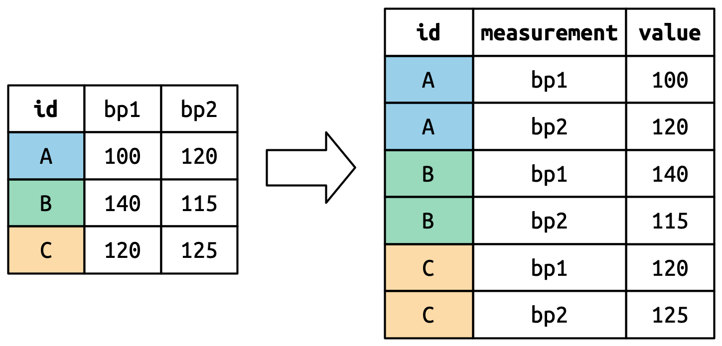
The column names become values in a new variable, whose name is defined by variable_name, as shown below. THey need to be repeated once for each row in the original dataset.

The column names of pivoted columns become values in a new column. The values need to be repeated once for each row of the original dataset.

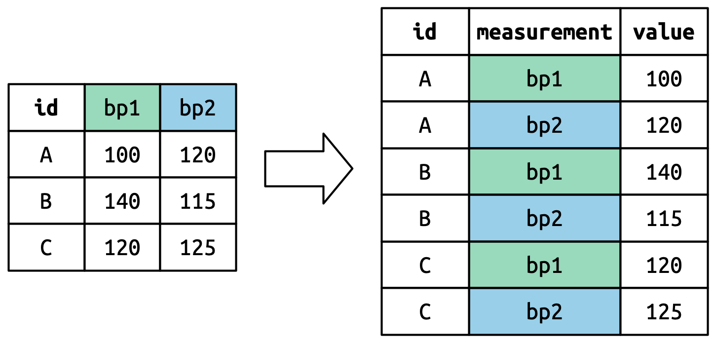
The cell values also become values in a new variable, with a name defined by values_name. They are unwound row by row, as shown below.

The number of values is preserved (not repeated), but unwound row-by-row.

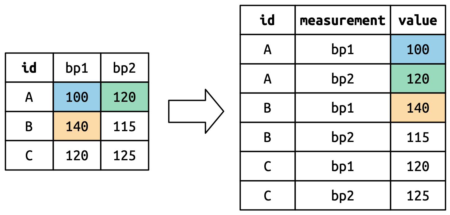
4.2.3 More variables in column names

A more challenging situation occurs when you have multiple pieces of information crammed into the column names, and you would like to store these in separate new variables. For example, take the who dataset, the source of table1 and friends you saw above:

who2 = pl.read_csv("data/who2.csv", null_values="")
who2

shape: (7_240, 58)

country	year	sp_m_014	sp_m_1524	sp_m_2534	sp_m_3544	sp_m_4554	sp_m_5564	sp_m_65	sp_f_014	sp_f_1524	sp_f_2534	sp_f_3544	sp_f_4554	sp_f_5564	sp_f_65	sn_m_014	sn_m_1524	sn_m_2534	sn_m_3544	sn_m_4554	sn_m_5564	sn_m_65	sn_f_014	sn_f_1524	sn_f_2534	sn_f_3544	sn_f_4554	sn_f_5564	sn_f_65	ep_m_014	ep_m_1524	ep_m_2534	ep_m_3544	ep_m_4554	ep_m_5564	ep_m_65	ep_f_014	ep_f_1524	ep_f_2534	ep_f_3544	ep_f_4554	ep_f_5564	ep_f_65	rel_m_014	rel_m_1524	rel_m_2534	rel_m_3544	rel_m_4554	rel_m_5564	rel_m_65	rel_f_014	rel_f_1524	rel_f_2534	rel_f_3544	rel_f_4554	rel_f_5564	rel_f_65
str	i64	i64	i64	i64	i64	i64	i64	i64	i64	i64	i64	i64	i64	i64	i64	i64	i64	i64	i64	i64	i64	i64	i64	i64	i64	i64	i64	i64	i64	i64	i64	i64	i64	i64	i64	i64	i64	i64	i64	i64	i64	i64	i64	i64	i64	i64	i64	i64	i64	i64	i64	i64	i64	i64	i64	i64	i64
"Afghanistan"	1980	null	null	null	null	null	null	null	null	null	null	null	null	null	null	null	null	null	null	null	null	null	null	null	null	null	null	null	null	null	null	null	null	null	null	null	null	null	null	null	null	null	null	null	null	null	null	null	null	null	null	null	null	null	null	null	null
"Afghanistan"	1981	null	null	null	null	null	null	null	null	null	null	null	null	null	null	null	null	null	null	null	null	null	null	null	null	null	null	null	null	null	null	null	null	null	null	null	null	null	null	null	null	null	null	null	null	null	null	null	null	null	null	null	null	null	null	null	null
"Afghanistan"	1982	null	null	null	null	null	null	null	null	null	null	null	null	null	null	null	null	null	null	null	null	null	null	null	null	null	null	null	null	null	null	null	null	null	null	null	null	null	null	null	null	null	null	null	null	null	null	null	null	null	null	null	null	null	null	null	null
"Afghanistan"	1983	null	null	null	null	null	null	null	null	null	null	null	null	null	null	null	null	null	null	null	null	null	null	null	null	null	null	null	null	null	null	null	null	null	null	null	null	null	null	null	null	null	null	null	null	null	null	null	null	null	null	null	null	null	null	null	null
…	…	…	…	…	…	…	…	…	…	…	…	…	…	…	…	…	…	…	…	…	…	…	…	…	…	…	…	…	…	…	…	…	…	…	…	…	…	…	…	…	…	…	…	…	…	…	…	…	…	…	…	…	…	…	…	…	…
"Zimbabwe"	2010	150	710	2208	1682	761	350	252	173	974	2185	1283	490	265	171	1826	821	3342	3270	1545	882	864	1732	1282	4013	2851	1377	789	563	270	243	902	868	418	229	192	220	319	1058	677	338	181	146	null	null	null	null	null	null	null	null	null	null	null	null	null	null
"Zimbabwe"	2011	152	784	2467	2071	780	377	278	174	1084	2161	1386	448	274	160	1364	596	2473	2813	1264	702	728	1271	947	2754	2216	962	587	495	250	195	746	796	342	172	172	209	318	802	640	284	137	129	null	null	null	null	null	null	null	null	null	null	null	null	null	null
"Zimbabwe"	2012	120	783	2421	2086	796	360	271	173	939	2053	1286	483	231	161	1169	613	2302	2657	1154	708	796	1008	888	2287	1957	829	516	432	233	214	658	789	331	178	182	208	319	710	579	228	140	143	null	null	null	null	null	null	null	null	null	null	null	null	null	null
"Zimbabwe"	2013	null	null	null	null	null	null	null	null	null	null	null	null	null	null	null	null	null	null	null	null	null	null	null	null	null	null	null	null	null	null	null	null	null	null	null	null	null	null	null	null	null	null	1315	1642	5331	5363	2349	1206	1208	1252	2069	4649	3526	1453	811	725

who2.glimpse()

Rows: 7240
Columns: 58
$ country    <str> 'Afghanistan', 'Afghanistan', 'Afghanistan', 'Afghanistan', 'Afghanistan', 'Afghanistan', 'Afghanistan', 'Afghanistan', 'Afghanistan', 'Afghanistan'
$ year       <i64> 1980, 1981, 1982, 1983, 1984, 1985, 1986, 1987, 1988, 1989
$ sp_m_014   <i64> None, None, None, None, None, None, None, None, None, None
$ sp_m_1524  <i64> None, None, None, None, None, None, None, None, None, None
$ sp_m_2534  <i64> None, None, None, None, None, None, None, None, None, None
$ sp_m_3544  <i64> None, None, None, None, None, None, None, None, None, None
$ sp_m_4554  <i64> None, None, None, None, None, None, None, None, None, None
$ sp_m_5564  <i64> None, None, None, None, None, None, None, None, None, None
$ sp_m_65    <i64> None, None, None, None, None, None, None, None, None, None
$ sp_f_014   <i64> None, None, None, None, None, None, None, None, None, None
$ sp_f_1524  <i64> None, None, None, None, None, None, None, None, None, None
$ sp_f_2534  <i64> None, None, None, None, None, None, None, None, None, None
$ sp_f_3544  <i64> None, None, None, None, None, None, None, None, None, None
$ sp_f_4554  <i64> None, None, None, None, None, None, None, None, None, None
$ sp_f_5564  <i64> None, None, None, None, None, None, None, None, None, None
$ sp_f_65    <i64> None, None, None, None, None, None, None, None, None, None
$ sn_m_014   <i64> None, None, None, None, None, None, None, None, None, None
$ sn_m_1524  <i64> None, None, None, None, None, None, None, None, None, None
$ sn_m_2534  <i64> None, None, None, None, None, None, None, None, None, None
$ sn_m_3544  <i64> None, None, None, None, None, None, None, None, None, None
$ sn_m_4554  <i64> None, None, None, None, None, None, None, None, None, None
$ sn_m_5564  <i64> None, None, None, None, None, None, None, None, None, None
$ sn_m_65    <i64> None, None, None, None, None, None, None, None, None, None
$ sn_f_014   <i64> None, None, None, None, None, None, None, None, None, None
$ sn_f_1524  <i64> None, None, None, None, None, None, None, None, None, None
$ sn_f_2534  <i64> None, None, None, None, None, None, None, None, None, None
$ sn_f_3544  <i64> None, None, None, None, None, None, None, None, None, None
$ sn_f_4554  <i64> None, None, None, None, None, None, None, None, None, None
$ sn_f_5564  <i64> None, None, None, None, None, None, None, None, None, None
$ sn_f_65    <i64> None, None, None, None, None, None, None, None, None, None
$ ep_m_014   <i64> None, None, None, None, None, None, None, None, None, None
$ ep_m_1524  <i64> None, None, None, None, None, None, None, None, None, None
$ ep_m_2534  <i64> None, None, None, None, None, None, None, None, None, None
$ ep_m_3544  <i64> None, None, None, None, None, None, None, None, None, None
$ ep_m_4554  <i64> None, None, None, None, None, None, None, None, None, None
$ ep_m_5564  <i64> None, None, None, None, None, None, None, None, None, None
$ ep_m_65    <i64> None, None, None, None, None, None, None, None, None, None
$ ep_f_014   <i64> None, None, None, None, None, None, None, None, None, None
$ ep_f_1524  <i64> None, None, None, None, None, None, None, None, None, None
$ ep_f_2534  <i64> None, None, None, None, None, None, None, None, None, None
$ ep_f_3544  <i64> None, None, None, None, None, None, None, None, None, None
$ ep_f_4554  <i64> None, None, None, None, None, None, None, None, None, None
$ ep_f_5564  <i64> None, None, None, None, None, None, None, None, None, None
$ ep_f_65    <i64> None, None, None, None, None, None, None, None, None, None
$ rel_m_014  <i64> None, None, None, None, None, None, None, None, None, None
$ rel_m_1524 <i64> None, None, None, None, None, None, None, None, None, None
$ rel_m_2534 <i64> None, None, None, None, None, None, None, None, None, None
$ rel_m_3544 <i64> None, None, None, None, None, None, None, None, None, None
$ rel_m_4554 <i64> None, None, None, None, None, None, None, None, None, None
$ rel_m_5564 <i64> None, None, None, None, None, None, None, None, None, None
$ rel_m_65   <i64> None, None, None, None, None, None, None, None, None, None
$ rel_f_014  <i64> None, None, None, None, None, None, None, None, None, None
$ rel_f_1524 <i64> None, None, None, None, None, None, None, None, None, None
$ rel_f_2534 <i64> None, None, None, None, None, None, None, None, None, None
$ rel_f_3544 <i64> None, None, None, None, None, None, None, None, None, None
$ rel_f_4554 <i64> None, None, None, None, None, None, None, None, None, None
$ rel_f_5564 <i64> None, None, None, None, None, None, None, None, None, None
$ rel_f_65   <i64> None, None, None, None, None, None, None, None, None, None

This dataset, collected by the World Health Organization, records information about tuberculosis diagnoses. There are two columns that are already variables and are easy to interpret: country and year. They are followed by 56 columns like sp_m_014, ep_m_4554, and rel_m_3544. If you stare at these columns for long enough, you’ll notice there’s a pattern. Each column name is made up of three pieces separated by _. The first piece, sp/rel/ep, describes the method used for the diagnosis, the second piece, m/f is the gender (coded as a binary variable in this dataset), and the third piece, 014/1524/2534/3544/4554/5564/65 is the age range (014 represents 0-14, for example).

So in this case, we have six pieces of information recorded in who2: the country and the year (already columns); the method of diagnosis, the gender category, and the age range category (contained in the other column names); and the count of patients in that category (cell values).

To organize these six pieces of information in six separate columns, first we use DataFrame.unpivot() like before, then we have to do some data wrangling using list expressions to split the information from the column names into separate columns:

1. Unpivot:

step1 = who2.unpivot(
    index=["country", "year"],
    variable_name="key",
    value_name="count"
)

step1

shape: (405_440, 4)

country	year	key	count
str	i64	str	i64
"Afghanistan"	1980	"sp_m_014"	null
"Afghanistan"	1981	"sp_m_014"	null
"Afghanistan"	1982	"sp_m_014"	null
"Afghanistan"	1983	"sp_m_014"	null
…	…	…	…
"Zimbabwe"	2010	"rel_f_65"	null
"Zimbabwe"	2011	"rel_f_65"	null
"Zimbabwe"	2012	"rel_f_65"	null
"Zimbabwe"	2013	"rel_f_65"	725

2. Split the key column into diagnosis, gender, and age columns:

step2 = step1.with_columns(
    pl.col("key").str.split("_")
)

step2

shape: (405_440, 4)

country	year	key	count
str	i64	list[str]	i64
"Afghanistan"	1980	["sp", "m", "014"]	null
"Afghanistan"	1981	["sp", "m", "014"]	null
"Afghanistan"	1982	["sp", "m", "014"]	null
"Afghanistan"	1983	["sp", "m", "014"]	null
…	…	…	…
"Zimbabwe"	2010	["rel", "f", "65"]	null
"Zimbabwe"	2011	["rel", "f", "65"]	null
"Zimbabwe"	2012	["rel", "f", "65"]	null
"Zimbabwe"	2013	["rel", "f", "65"]	725

3. Extract each list element into a new column:

step3 = step2.select(
    pl.col("country"),
    pl.col("year"),
    pl.col("key").list.get(0).alias("diagnosis"), # Polars also uses 0-indexing
    pl.col("key").list.get(1).alias("gender"),
    pl.col("key").list.get(2).alias("age"),
    pl.col("count")
)

step3

shape: (405_440, 6)

country	year	diagnosis	gender	age	count
str	i64	str	str	str	i64
"Afghanistan"	1980	"sp"	"m"	"014"	null
"Afghanistan"	1981	"sp"	"m"	"014"	null
"Afghanistan"	1982	"sp"	"m"	"014"	null
"Afghanistan"	1983	"sp"	"m"	"014"	null
…	…	…	…	…	…
"Zimbabwe"	2010	"rel"	"f"	"65"	null
"Zimbabwe"	2011	"rel"	"f"	"65"	null
"Zimbabwe"	2012	"rel"	"f"	"65"	null
"Zimbabwe"	2013	"rel"	"f"	"65"	725

All together:

(
    who2.unpivot(
        index=["country", "year"], variable_name="key", value_name="count"
    )
    .with_columns(
        pl.col("key").str.split("_")
    )
    .select(
        pl.col("country"),
        pl.col("year"),
        pl.col("key").list.get(0).alias("diagnosis"),
        pl.col("key").list.get(1).alias("gender"),
        pl.col("key").list.get(2).alias("age"),
        pl.col("count")
    )
)

While the above steps break down the process to understand easier, here is a more concise, albeit more advanced, way to achieve the same results:

(
    who2.unpivot(
        index=["country", "year"], 
        variable_name="key", 
        value_name="count"
    )
    .with_columns(
        pl.col("key")
        .str.split("_")
        .list.to_struct(fields=["diagnosis", "gender", "age"])
    )
    .unnest("key")
)

shape: (405_440, 6)

country	year	diagnosis	gender	age	count
str	i64	str	str	str	i64
"Afghanistan"	1980	"sp"	"m"	"014"	null
"Afghanistan"	1981	"sp"	"m"	"014"	null
"Afghanistan"	1982	"sp"	"m"	"014"	null
"Afghanistan"	1983	"sp"	"m"	"014"	null
…	…	…	…	…	…
"Zimbabwe"	2010	"rel"	"f"	"65"	null
"Zimbabwe"	2011	"rel"	"f"	"65"	null
"Zimbabwe"	2012	"rel"	"f"	"65"	null
"Zimbabwe"	2013	"rel"	"f"	"65"	725

Conceptually, this is only a minor variation on the simpler case you’ve already seen. The figure below shows the basic idea: now, instead of the column names pivoting into a single column, they pivot into multiple columns.

Pivoting columns with multiple pieces of information in the names means that each column name now fills in values in multiple output columns.

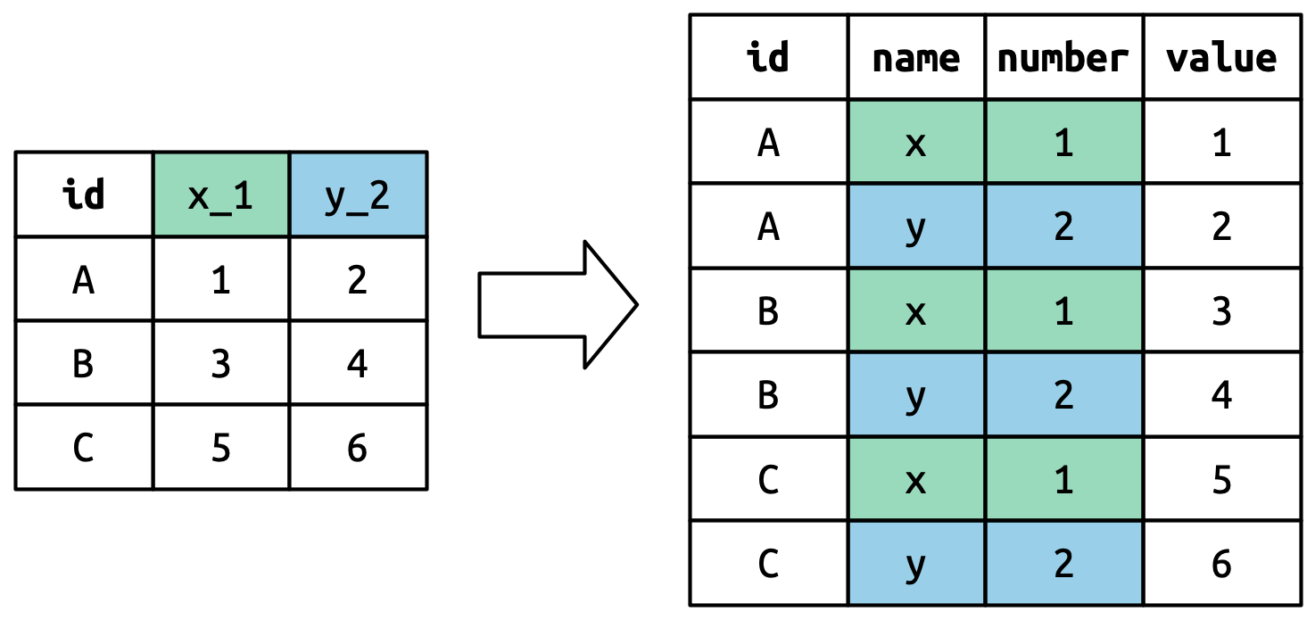
4.3 Widening data

So far we’ve used DataFrame.unpivot() to solve the common class of problems where values have ended up in column names. Next we’ll pivot (HA HA) to DataFrame.pivot(), which makes datasets wider by increasing columns and reducing rows and helps when one observation is spread across multiple rows. This seems to arise less commonly in the wild, but it does seem to crop up a lot when dealing with governmental data.

We’ll start by looking at cms_patient_experience, a dataset from the Centers of Medicare and Medicaid services that collects data about patient experiences:

cms_patient_experience = pl.read_csv(
    "data/cms_patient_experience.csv", 
    schema_overrides={"org_pac_id": pl.String}
)

cms_patient_experience

shape: (500, 5)

org_pac_id	org_nm	measure_cd	measure_title	prf_rate
str	str	str	str	i64
"0446157747"	"USC CARE MEDICAL GROUP INC"	"CAHPS_GRP_1"	"CAHPS for MIPS SSM: Getting Ti…	63
"0446157747"	"USC CARE MEDICAL GROUP INC"	"CAHPS_GRP_2"	"CAHPS for MIPS SSM: How Well P…	87
"0446157747"	"USC CARE MEDICAL GROUP INC"	"CAHPS_GRP_3"	"CAHPS for MIPS SSM: Patient's …	86
"0446157747"	"USC CARE MEDICAL GROUP INC"	"CAHPS_GRP_5"	"CAHPS for MIPS SSM: Health Pro…	57
…	…	…	…	…
"9931011434"	"PATIENT FIRST RICHMOND MEDICAL…	"CAHPS_GRP_2"	"CAHPS for MIPS SSM: How Well P…	null
"9931011434"	"PATIENT FIRST RICHMOND MEDICAL…	"CAHPS_GRP_3"	"CAHPS for MIPS SSM: Patient's …	null
"9931011434"	"PATIENT FIRST RICHMOND MEDICAL…	"CAHPS_GRP_5"	"CAHPS for MIPS SSM: Health Pro…	45
"9931011434"	"PATIENT FIRST RICHMOND MEDICAL…	"CAHPS_GRP_12"	"CAHPS for MIPS SSM: Stewardshi…	19

The core unit being studied is an organization, but each organization is spread across six rows, with one row for each measurement taken in the survey organization. We can see the complete set of values for measure_cd and measure_title by using DataFrame.unique().select():

cols = ["measure_cd", "measure_title"]

cms_patient_experience.unique(subset=cols).select(cols).sort(cols)

shape: (6, 2)

measure_cd	measure_title
str	str
"CAHPS_GRP_1"	"CAHPS for MIPS SSM: Getting Ti…
"CAHPS_GRP_12"	"CAHPS for MIPS SSM: Stewardshi…
"CAHPS_GRP_2"	"CAHPS for MIPS SSM: How Well P…
"CAHPS_GRP_3"	"CAHPS for MIPS SSM: Patient's …
"CAHPS_GRP_5"	"CAHPS for MIPS SSM: Health Pro…
"CAHPS_GRP_8"	"CAHPS for MIPS SSM: Courteous …

Neither of these columns will make particularly great variable names: measure_cd doesn’t hint at the meaning of the variable and measure_title is a long sentence containing spaces. We’ll use measure_cd as the source for our new column names for now, but in a real analysis you might want to create your own variable names that are both short and meaningful.

DataFrame.pivot() has a similar, but different, interface than DataFrame.unpivot(): you still select the index columns (the columns that remain), but now you select which column the values will come from, and which column the names come from (on).

cms_patient_experience.pivot(
    index=["org_pac_id", "org_nm"],
    on=["measure_cd"], # Notice we don't use `measure_title`
    values="prf_rate"
)

shape: (95, 8)

org_pac_id	org_nm	CAHPS_GRP_1	CAHPS_GRP_2	CAHPS_GRP_3	CAHPS_GRP_5	CAHPS_GRP_8	CAHPS_GRP_12
str	str	i64	i64	i64	i64	i64	i64
"0446157747"	"USC CARE MEDICAL GROUP INC"	63	87	86	57	85	24
"0446162697"	"ASSOCIATION OF UNIVERSITY PHYS…	59	85	83	63	88	22
"0547164295"	"BEAVER MEDICAL GROUP PC"	49	null	75	44	73	12
"0749333730"	"CAPE PHYSICIANS ASSOCIATES PA"	67	84	85	65	82	24
…	…	…	…	…	…	…	…
"9830008770"	"WASHINGTON UNIVERSITY"	65	null	null	61	null	28
"9830093640"	"COOPERATIVE HEALTHCARE SERVICE…	65	87	78	52	null	25
"9830094515"	"SUTTER VALLEY MEDICAL FOUNDATI…	60	null	88	55	null	24
"9931011434"	"PATIENT FIRST RICHMOND MEDICAL…	80	null	null	45	null	19

4.3.1 How does DataFrame.pivot() work?

To understand how DataFrame.pivot() works, let’s again start with a very simple dataset. This time we have two patients with ids A and B, we have three blood pressure measurements on patient A and two on patient B:

df = pl.from_dict({
    "id": ["A", "B", "B", "A", "A"],
    "measurement": ["bp1", "bp1", "bp2", "bp2", "bp3"],
    "value": [100, 140, 115, 120, 105]
})

df

shape: (5, 3)

id	measurement	value
str	str	i64
"A"	"bp1"	100
"B"	"bp1"	140
"B"	"bp2"	115
"A"	"bp2"	120
"A"	"bp3"	105

We’ll take the values from the value column and the names from the measurement column:

df.pivot(on="measurement", values="value") # unused cols get put in `index`

shape: (2, 4)

id	bp1	bp2	bp3
str	i64	i64	i64
"A"	100	120	105
"B"	140	115	null

To begin the process, DataFrame.pivot() needs to first figure out what will go in the rows and columns. The new column names will be the unique values of measurement.

df.select("measurement").unique()

shape: (3, 1)

measurement
str
"bp2"
"bp3"
"bp1"

By default, the rows in the output are determined by all the variables that aren’t going into the new names or values. These are called the index columns. Here there is only one column, but in general there can be any number.

df.select(pl.exclude("measurement", "value")).unique()

shape: (2, 1)

id
str
"A"
"B"

DataFrame.pivot() then combines these results to generate an empty data frame:

df.select(pl.exclude("measurement", "value")).unique().with_columns(
    x=pl.lit(None), y=pl.lit(None), z=pl.lit(None)
)

shape: (2, 4)

id	x	y	z
str	null	null	null
"A"	null	null	null
"B"	null	null	null

It then fills in all the missing values using the data in the input. In this case, not every cell in the output has a corresponding value in the input as there’s no third blood pressure measurement for patient B, so that cell remains missing.

4.3.2 Data and variable names in the column headers

We will now see an example where we need to unpivot and pivot in the same set of steps to tidy our data. This step up in complexity is when the column names include a mix of variable values and variable names. For example, take the household dataset:

household = pl.from_dict({
    "family": [1, 2, 3, 4, 5],
    "dob_child1": ["1998-11-26", "1996-06-22", "2002-07-11", "2004-10-10", "2000-12-05"],
    "dob_child2": ["2000-01-29", None, "2004-04-05", "2009-08-27", "2005-02-28"],
    "name_child1": ["Susan", "Mark", "Sam", "Craig", "Parker"],
    "name_child2": ["Jose", None, "Seth", "Khai", "Gracie"]
}).with_columns(
    cs.starts_with("dob").str.to_date()
)

household

shape: (5, 5)

family	dob_child1	dob_child2	name_child1	name_child2
i64	date	date	str	str
1	1998-11-26	2000-01-29	"Susan"	"Jose"
2	1996-06-22	null	"Mark"	null
3	2002-07-11	2004-04-05	"Sam"	"Seth"
4	2004-10-10	2009-08-27	"Craig"	"Khai"
5	2000-12-05	2005-02-28	"Parker"	"Gracie"

This dataset contains data about five families, with the names and dates of birth of up to two children. The new challenge in this dataset is that the column names contain the names of two variables (dob, name) and the values of another (child, with values 1 or 2).

(
    # First, unpivot the data frame to create rows for each family-column combination
    household.unpivot(index="family")

    # Extract the base column name (dob/name) and the child number
    .with_columns(
        pl.col("variable")
        .str.split("_")
        .list.to_struct(fields=["base_col", "child"])
    )
    .unnest("variable")

    # Pivot the data to create separate columns for each base_col (dob, name)
    .pivot(index=["family", "child"], on="base_col", values="value")

    # Filter out rows with null values
    .drop_nulls()

    # Clean up results
    .sort(["family", "child"])
    .with_columns(pl.col("dob").str.to_date())
)

shape: (9, 4)

family	child	dob	name
i64	str	date	str
1	"child1"	1998-11-26	"Susan"
1	"child2"	2000-01-29	"Jose"
2	"child1"	1996-06-22	"Mark"
3	"child1"	2002-07-11	"Sam"
…	…	…	…
4	"child1"	2004-10-10	"Craig"
4	"child2"	2009-08-27	"Khai"
5	"child1"	2000-12-05	"Parker"
5	"child2"	2005-02-28	"Gracie"

We use DataFrame.drop_nulls() since the shape of the input forces the creation of explicit missing variables (e.g., for families that only have one child).

4.4 Summary

In this section, you learned about tidy data: data that has variables in columns and observations in rows. Tidy data makes working in the Polars easier, because it’s a consistent structure understood by most functions, the main challenge is transforming the data from whatever structure you receive it in to a tidy format. To that end, you learned about DataFrame.unpivot() and DataFrame.pivot() which allow you to tidy up many untidy datasets.

Another challenge is that, for a given dataset, it can be impossible to label the longer or the wider version as the “tidy” one. This is partly a reflection of our definition of tidy data, where we said tidy data has one variable in each column, but we didn’t actually define what a variable is (and it’s surprisingly hard to do so). It’s totally fine to be pragmatic and to say a variable is whatever makes your analysis easiest. So if you’re stuck figuring out how to do some computation, consider switching up the organization of your data; don’t be afraid to untidy, transform, and re-tidy as needed!

5 Data import & export

Working with data provided by Python packages is a great way to learn data science tools, but at some point, you’ll want to apply what you’ve learned to your own data. In this section, you’ll learn the basics of reading data files into Python and how to export them for others (or yourself in the future) to use.

Specifically, this chapter will focus on reading plain-text rectangular files. We’ll start with practical advice for handling features like column names, types, and missing data. You will then learn about reading data from multiple files at once and writing data from Python to a file. Finally, you’ll learn how to handcraft data frames in Python, and export them with Polars functions.

import io # we'll use this to "create" CSVs within Python examples

5.1 Reading data from a file

To begin, we’ll focus on the most common rectangular data file type: CSV, which is short for comma-separated values. Here is what a simple CSV file looks like. The first row, commonly called the header row, gives the column names, and the following six rows provide the data. The columns are separated, aka delimited, by commas.

Student ID,Full Name,favourite.food,mealPlan,AGE
1,Sunil Huffmann,Strawberry yoghurt,Lunch only,4
2,Barclay Lynn,French fries,Lunch only,5
3,Jayendra Lyne,N/A,Breakfast and lunch,7
4,Leon Rossini,Anchovies,Lunch only,
5,Chidiegwu Dunkel,Pizza,Breakfast and lunch,five
6,Güvenç Attila,Ice cream,Lunch only,6

The following table shows a representation of the same data as a table:

Student ID	Full Name	favourite.food	mealPlan	AGE
1	Sunil Huffmann	Strawberry yoghurt	Lunch only	4
2	Barclay Lynn	French fries	Lunch only	5
3	Jayendra Lyne	N/A	Breakfast and lunch	7
4	Leon Rossini	Anchovies	Lunch only	NULL
5	Chidiegwu Dunkel	Pizza	Breakfast and lunch	five
6	Guvenc Attila	Ice cream	Lunch only	6

We can read this file into Python using pl.read_csv(). The first argument is the most important: the path to the file. You can think about the path as the address of the file: the file is called students.csv and it lives in the data folder.

students = pl.read_csv("data/students.csv")

The code above will work if you have the students.csv file in a data folder in your project. You can also read it directly from a URL:

students = pl.read_csv("https://raw.githubusercontent.com/hadley/r4ds/main/data/students.csv")

When you run pl.read_csv(), Polars will scan the file and automatically infer column types based on the data it contains. Polars doesn’t print a detailed message about column specifications by default, but you can examine the schema to see the inferred types:

students.schema.to_frame()

shape: (0, 5)

Student ID	Full Name	favourite.food	mealPlan	AGE
i64	str	str	str	str

5.1.1 Practical advice

Once you read data in, the first step usually involves transforming it in some way to make it easier to work with in the rest of your analysis. Let’s take another look at the students data with that in mind.

students

shape: (6, 5)

Student ID	Full Name	favourite.food	mealPlan	AGE
i64	str	str	str	str
1	"Sunil Huffmann"	"Strawberry yoghurt"	"Lunch only"	"4"
2	"Barclay Lynn"	"French fries"	"Lunch only"	"5"
3	"Jayendra Lyne"	"N/A"	"Breakfast and lunch"	"7"
4	"Leon Rossini"	"Anchovies"	"Lunch only"	null
5	"Chidiegwu Dunkel"	"Pizza"	"Breakfast and lunch"	"five"
6	"Güvenç Attila"	"Ice cream"	"Lunch only"	"6"

In the favourite.food column, there’s an entry “N/A” that should be interpreted as a real None that Python will recognize as “not available”. This is something we can address using the null_values argument. By default, Polars only recognizes empty strings and the string “null” (case-insensitive) as missing values.

students = pl.read_csv(
    "data/students.csv", 
    null_values=["N/A", ""]
)

students

shape: (6, 5)

Student ID	Full Name	favourite.food	mealPlan	AGE
i64	str	str	str	str
1	"Sunil Huffmann"	"Strawberry yoghurt"	"Lunch only"	"4"
2	"Barclay Lynn"	"French fries"	"Lunch only"	"5"
3	"Jayendra Lyne"	null	"Breakfast and lunch"	"7"
4	"Leon Rossini"	"Anchovies"	"Lunch only"	null
5	"Chidiegwu Dunkel"	"Pizza"	"Breakfast and lunch"	"five"
6	"Güvenç Attila"	"Ice cream"	"Lunch only"	"6"

You might also notice that Student ID and Full Name columns contain spaces, which can make them awkward to work with in code. In Polars, you can refer to these columns using either bracket notation or with the . accessor, but the latter won’t work with spaces or special characters:

# Works with spaces
first_student_name = students["Full Name"][0]
print(first_student_name)

# Won't work with spaces
first_student_name = students.Full Name[0]  # Syntax error!

  Cell In[94], line 6
    first_student_name = students.Full Name[0]  # Syntax error!
                                       ^
SyntaxError: invalid syntax

It’s often a good idea to rename these columns to follow Python naming conventions. Here’s how you can rename specific columns:

students = students.rename({
    "Student ID": "student_id",
    "Full Name": "full_name"
})

students

shape: (6, 5)

student_id	full_name	favourite.food	mealPlan	AGE
i64	str	str	str	str
1	"Sunil Huffmann"	"Strawberry yoghurt"	"Lunch only"	"4"
2	"Barclay Lynn"	"French fries"	"Lunch only"	"5"
3	"Jayendra Lyne"	null	"Breakfast and lunch"	"7"
4	"Leon Rossini"	"Anchovies"	"Lunch only"	null
5	"Chidiegwu Dunkel"	"Pizza"	"Breakfast and lunch"	"five"
6	"Güvenç Attila"	"Ice cream"	"Lunch only"	"6"

An alternative approach is to use a function to clean all column names at once. Polars doesn’t have a built-in function for this, but we can use a special shortcut called a lambda function to do this in one line. Think of a lambda function as a mini-function that you can write directly where you need it, without having to define it separately. It’s like giving Polars quick instructions on how to transform each column name.

students = (
    students.rename(
        lambda col_name: col_name.lower().replace(" ", "_").replace(".", "_")
    )
)

With this code, we are telling Polars to take each column name (not the values of the columns), call it col, and do these three things to it:

1. Convert it to lowercase
2. Replace any spaces with underscores
3. Replace any periods with underscores

Note that these are the string methods we learned earlier in this course, not functions that come from Polars. col_name has the type str.

Like in for loops, it doesn’t matter what the looping (or lambda) variable is called. I just called it col_name because that is what we are effecting. I could’ve also called it x and it would work the same:

students = (
    students.rename(
        lambda x: x.lower().replace(" ", "_").replace(".", "_")
    )
)

If you wanted to use a regular function, you could do something like this:

def clean_col_name(col_name):
    return col_name.lower().replace(" ", "_").replace(".", "_")

students = students.rename(clean_column_name) 
# Note: no parentheses here, we're passing the function itself

When would you want to use a named/user-defined function over a lambda function? It comes down to how many times you would repeat the steps. If you are working with only one data frame, a lambda function might be quicker to write, but if you are going to clean multiple data frames in the same script, creating a named function to use over again would be the better method.

Note

You can use this code snippet to help you with your labs and tests. You don’t need to fully understand lambda functions for this course, but you can think of this specific pattern as a helpful ‘recipe’ for cleaning column names in one step while keeping your code clean and readable. If you ever need to customize how column names are cleaned, you can just adjust what happens inside the lambda function. The Polars documentation for DataFrame.rename() has another example using lambda functions to rename columns.

Another common task after reading in data is to consider variable types. For example, meal_plan is a categorical variable with a known set of possible values, which in Python should be represented as a category:

students = students.with_columns(
    pl.col("mealplan").cast(pl.Categorical)
)
students

shape: (6, 5)

student_id	full_name	favourite_food	mealplan	age
i64	str	str	cat	str
1	"Sunil Huffmann"	"Strawberry yoghurt"	"Lunch only"	"4"
2	"Barclay Lynn"	"French fries"	"Lunch only"	"5"
3	"Jayendra Lyne"	null	"Breakfast and lunch"	"7"
4	"Leon Rossini"	"Anchovies"	"Lunch only"	null
5	"Chidiegwu Dunkel"	"Pizza"	"Breakfast and lunch"	"five"
6	"Güvenç Attila"	"Ice cream"	"Lunch only"	"6"

Before you analyze this dataset, you’ll probably want to fix the age column. Currently, age contains mixed types because one observation is typed out as “five” instead of the number 5:

students = students.with_columns(
    age=pl.when(pl.col("age") == "five")
    .then(pl.lit(5))
    .otherwise(pl.col("age").cast(pl.Int64, strict=False))
) # This is conceptually very similar to Python's built in if-elif-else

students

shape: (6, 5)

student_id	full_name	favourite_food	mealplan	age
i64	str	str	cat	i64
1	"Sunil Huffmann"	"Strawberry yoghurt"	"Lunch only"	4
2	"Barclay Lynn"	"French fries"	"Lunch only"	5
3	"Jayendra Lyne"	null	"Breakfast and lunch"	7
4	"Leon Rossini"	"Anchovies"	"Lunch only"	null
5	"Chidiegwu Dunkel"	"Pizza"	"Breakfast and lunch"	5
6	"Güvenç Attila"	"Ice cream"	"Lunch only"	6

The Polars code above uses a conditional expression with when(), then(), and otherwise() to handle the special case, then attempts to cast the column to a floating-point number. The strict=False parameter tells Polars to convert values that can be parsed as numbers and set the rest to None.

5.1.2 Other arguments

Usually, pl.read_csv() uses the first line of the data for the column names, which is a very common convention. But it’s not uncommon for a few lines of metadata to be included at the top of the file. You can use skip_rows to skip the first n lines:

csv_data = """The first line of metadata
The second line of metadata
x,y,z 
1,2,3"""

pl.read_csv(io.StringIO(csv_data), skip_rows=2)

shape: (1, 3)

x	y	z
i64	i64	i64
1	2	3

In other cases, the data might not have column names. You can use has_header=False to tell Polars not to treat the first row as headings:

csv_data = """1,2,3
4,5,6"""

pl.read_csv(io.StringIO(csv_data), has_header=False)

shape: (2, 3)

column_1	column_2	column_3
i64	i64	i64
1	2	3
4	5	6

By default, Polars will name the columns “column_1”, “column_2”, etc. You can provide your own column names with the new_columns parameter:

csv_data = """1,2,3
4,5,6"""

pl.read_csv(
    io.StringIO(csv_data), 
    has_header=False,
    new_columns=["x", "y", "z"]
)

shape: (2, 3)

x	y	z
i64	i64	i64
1	2	3
4	5	6

These arguments are all you need to know to read the majority of CSV files that you’ll encounter in practice. (For the rest, you’ll need to carefully inspect your .csv file and read the documentation for pl.read_csv()’s many other arguments.)

5.1.3 Other file types

Once you’ve mastered read_csv(), using Polars’ other functions is straightforward; it’s just a matter of knowing which function to reach for:

• read_csv() reads comma-separated files.
• read_csv() can also read semicolon-separated files by setting separator=";".
• read_csv() can read tab-delimited files by setting separator="\t", or you can use the alias read_tsv().
• read_csv() can read files with any delimiter by setting the separator parameter.
• read_ndjson() reads newline-delimited JSON files.
• read_parquet() reads Apache Parquet files, a columnar storage format that is typically faster and more space-efficient than CSV.
• read_ipc() or read_arrow() reads Arrow IPC files, which provide high-performance interoperability between different systems.
• read_excel() reads Excel files (learn more about the different Excel features here).
• read_avro() reads Avro files.

5.2 Controlling column types

A CSV file doesn’t contain any information about the type of each variable (i.e., whether it’s a boolean, number, string, etc.), so Polars will try to guess the type. This section describes how the guessing process works, how to resolve some common problems that cause it to fail, and how to supply the column types yourself.

5.2.1 Guessing types

Polars uses a heuristic to figure out the column types. By default, it samples a certain number of rows from the file and tries to infer the type based on the values it sees. You can control this with the infer_schema_length parameter.

The type inference generally follows these rules: - If values are “true” or “false” (case-insensitive), it’s a boolean. - If values are all integers, it’s an integer type. - If values have decimals but are all numeric, it’s a floating-point type. - If values match a date or datetime pattern, it’s a date or datetime type. - Otherwise, it’s a string type.

You can see that behavior with a simple example:

csv_data = """logical,numeric,date,string
TRUE,1,2021-01-15,abc
false,4.5,2021-02-15,def
T,Inf,2021-02-16,ghi"""

pl.read_csv(io.StringIO(csv_data))

shape: (3, 4)

logical	numeric	date	string
str	str	str	str
"TRUE"	"1"	"2021-01-15"	"abc"
"false"	"4.5"	"2021-02-15"	"def"
"T"	"Inf"	"2021-02-16"	"ghi"

This heuristic works well if you have a clean dataset, but in real life, you’ll encounter a variety of challenges that require special handling.

5.2.2 Missing values, column types, and problems

The most common way column detection fails is that a column contains unexpected values, and you get a string column instead of a more specific type. One of the most common causes is a missing value recorded using something other than the None that Polars expects.

Take this simple 1-column CSV file as an example:

simple_csv = """x
10
.
20
30"""

# Read without specifying null values
pl.read_csv(io.StringIO(simple_csv))

shape: (4, 1)

x
str
"10"
"."
"20"
"30"

If we read it without any additional arguments, x becomes a string column. In this very small example, you can easily see the missing value .. But what if you have thousands of rows with only a few missing values represented by .s scattered throughout?

In Polars, you can specify the column type and tell it what values should be treated as null:

pl.read_csv(
    io.StringIO(simple_csv),
    schema_overrides={"x": pl.Int64},
    null_values=["."],
)

shape: (4, 1)

x
i64
10
null
20
30

5.2.3 Column types

Polars provides many data types that you can specify:

• pl.Boolean: For logical values (True/False)
• pl.Int8, pl.Int16, pl.Int32, pl.Int64: For integers of different sizes
• pl.UInt8, pl.UInt16, pl.UInt32, pl.UInt64: For unsigned integers (positive only)
• pl.Float32, pl.Float64: For floating-point numbers
• pl.Decimal: For precise decimal arithmetic
• pl.Utf8: For string data
• pl.Categorical: For categorical (factor) data
• pl.Date, pl.Time, pl.Datetime: For date and time data
• pl.Object: For Python objects that don’t fit the other types
• pl.Binary: For binary data
• pl.Struct: For nested data structures

You can specify column types in two ways:

1. Using the schema or schema_overrides parameter when reading data
2. Using cast() to convert columns after reading

# Specify types when reading
csv_data = """x,y,z
1,2,3"""

df = pl.read_csv(
    io.StringIO(csv_data),
    schema_overrides={
        "x": pl.Int32,
        "y": pl.Float64,
        "z": pl.Utf8
    }
)
print(df.schema)

# Or convert after reading
df = pl.read_csv(io.StringIO(csv_data))
df = df.with_columns([
    pl.col("x").cast(pl.Int32),
    pl.col("y").cast(pl.Float64),
    pl.col("z").cast(pl.Utf8)
])
print(df.schema)

Schema({'x': Int32, 'y': Float64, 'z': String})
Schema({'x': Int32, 'y': Float64, 'z': String})

You can also specify a schema for all columns at once:

schema = {"x": pl.Int32, "y": pl.Float64, "z": pl.Utf8}
df = pl.read_csv(io.StringIO(csv_data), schema=schema)
print(df.schema)

Schema({'x': Int32, 'y': Float64, 'z': String})

If you want to select only specific columns when reading a file, you can use the columns parameter:

df = pl.read_csv(io.StringIO(csv_data), columns=["x"])
print(df)

shape: (1, 1)
┌─────┐
│ x   │
│ --- │
│ i64 │
╞═════╡
│ 1   │
└─────┘

5.3 Reading data from multiple files

Sometimes your data is split across multiple files instead of being contained in a single file. For example, you might have sales data for multiple months, with each month’s data in a separate file: 01-sales.csv for January, 02-sales.csv for February, and 03-sales.csv for March.

With Polars, you can read these files one by one and then concatenate them:

# List of sales files
sales_files = [
    "data/01-sales.csv",
    "data/02-sales.csv",
    "data/03-sales.csv"
]

# Read and concatenate via list comprehension
dfs = [pl.read_csv(file).with_columns(pl.lit(os.path.basename(file)).alias("file")) 
       for file in sales_files]
sales = pl.concat(dfs)

Tip

This method uses something called List Comprehension, which you can learn more about here. We won’t need these techniques for this class, but you should be aware of them.

You can download these files from the URLs manually, or read them directly with Polars:

sales_files = [
    "https://pos.it/r4ds-01-sales",
    "https://pos.it/r4ds-02-sales",
    "https://pos.it/r4ds-03-sales"
]

dfs = [pl.read_csv(file).with_columns(pl.lit(file).alias("file")) 
       for file in sales_files]
sales = pl.concat(dfs)

If you have many files you want to read in, you can use the glob module to find the files by matching a pattern:

import glob

sales_files = glob.glob("data/*-sales.csv")
sales_files

5.4 Writing to a file

Polars provides several functions for writing data to disk. The most common are write_csv() and write_parquet(). The most important arguments to these functions are the DataFrame to save and the file path where you want to save it.

students.write_csv("students.csv")

Note that the variable type information you set up is lost when you save to CSV because you’re starting over with reading from a plain text file. This makes CSVs somewhat unreliable for caching interim results. You need to recreate the column specification every time you load in.

There are two better alternative is Parquet files. These maintain the column types and are generally faster and more space-efficient.

students.write_parquet("students.parquet")
parquet_students = pl.read_parquet("students.parquet")

Parquet is becoming more common in use with data sciences, but they have not caught on with more business based analytical tools like Excel, Tableau, & Power BI, so CSVs still reign supreme.

5.5 Data entry

Sometimes you’ll need to assemble a DataFrame “by hand” with a little data entry in your Python script. Polars provides a simple way to create data frames from dictionaries where each key is a column name and each value is a list of values:

df = pl.DataFrame({
    "x": [1, 2, 5],
    "y": ["h", "m", "g"],
    "z": [0.08, 0.83, 0.60]
})

df

shape: (3, 3)

x	y	z
i64	str	f64
1	"h"	0.08
2	"m"	0.83
5	"g"	0.6

You can also create a data frame from a list of dictionaries, where each dictionary represents a row:

df = pl.DataFrame([
    {"x": 1, "y": "h", "z": 0.08},
    {"x": 2, "y": "m", "z": 0.83},
    {"x": 5, "y": "g", "z": 0.60}
])

df

shape: (3, 3)

x	y	z
i64	str	f64
1	"h"	0.08
2	"m"	0.83
5	"g"	0.6

5.6 Summary

In this section, you’ve learned how to load CSV files with Polars’ pl.read_csv() and how to do your own data entry by creating DataFrames from dictionaries and lists. You’ve learned how CSV files work, some of the problems you might encounter, and how to overcome them.

You’ll revisit data import in various formats throughout your Python data science journey, including Excel files, databases, Parquet files, JSON, and data from websites.

Polars is an excellent choice for data handling, as it’s designed to take advantage of modern hardware through parallel processing and memory efficiency. As you become more familiar with Python data science tools, you’ll appreciate Polars’ performance benefits and elegant API design.

6 Exercises

1. Does it matter what order you used DataFrame.filter() and DataFrame.sort() if you’re using both? Why/why not? Think about the results and how much work the functions would have to do.

2. What happens if you specify the name of the same variable multiple times in a DataFrame.select() call?

3. Using the penguins dataset, make a scatter plot of bill_depth_mm vs. bill_length_mm. That is, make a scatter plot with bill_depth_mm on the y-axis and bill_length_mm on the x-axis. Describe the relationship between these two variables.

4. From the flights dataset, compare dep_time, sched_dep_time, and dep_delay. How would you expect those three numbers to be related?

5. In a single pipeline for each condition, find all flights that meet the condition:

   • Had an arrival delay of two or more hours
   • Flew to Houston (IAH or HOU)
   • Were operated by United, American, or Delta
   • Departed in summer (July, August, and September)
   • Arrived more than two hours late but didn’t leave late
   • Were delayed by at least an hour, but made up over 30 minutes in flight

6. Find the flights that are most delayed upon departure from each destination.

7. How do delays vary over the course of the day? Illustrate your answer with a plot.